Region 6 - USDA Forest Service
A Guide to the Interpretation and
Use of the DecAID Advisor
June, 2006
Latest update: September, 2017
For use with:
DecAID version 3.0
An Advisory Tool for Managing Snags and Down Wood
In Forests of Washington and Oregon
Introduction
This Guide accompanies DecAID versions 3.0 (September 2017), 2.20 (January 2012), 2.10 (January 2009) and 2.0 (January 2006) that replaces DecAID Version 1.10. This Guide does not apply to any ongoing planning efforts which utilize previous versions
A major update of DecAID occured with version 2.0, utilizing new wildlife habitat data and reflecting user experience gained in DecAID version 1.10. Five factors mark the major changes between DecAID and DecAID Version 1.10:
- updated Wildlife Habitat data (through December 2005);
- better landscape scale discussion in the narrative;
- clarifications of the Cautions and Caveats to improve user understanding;
- addition of the Lodgepole Pine Wildlife Habitat Type;
- creation of a separate Post-fire Structural Condition Class.
DecAID version 2.10 included additional information from recent literature and data, through October 2008, and a move of the web site from FS Domino Server to WWW. DecAID version 2.20 includes additional information from recent literature and data, through December 2011. DecAID version 3.0 (hereinafter referred to as DecAID) features an upgraded web site design to better use new web-based technologies, an updated and re-analyzed vegetation inventory data, redefined Structural Conditions Class to Successional/Structural Class (S-Class) with definitions and queries that better reflected wildlife use of habitats, and additional information from recent literature and data, through December 2016. See Version History for a complete description of changes made to DecAID as versions have been updated.
What is DecAID?
At its most basic level, the DecAID Advisor is a compilation of the best available science on the management of dead wood in forests of the Pacific Northwest. DecAID is not a model or cook-book that will give you a simple answer to this complex issue.
DecAID is an Internet-based summary, synthesis, and integration (a "meta-analysis") of the best available science: published scientific literature, research data, wildlife databases, forest inventory databases, and expert judgment and experience. The information presented on wildlife species use of snags and down wood is based entirely on scientific field research and does not rely on modeling wildlife populations. DecAID offers ways of estimating or evaluating sizes and densities or amounts of dead wood that provide habitat for many species and ecological processes.
DecAID is not a viability assessment. A viability analysis will require an assessment of other factors that may be impacting species populations.
What can DecAID do for you?
DecAID can:
- help managers evaluate effects of forest conditions and existing or proposed management activities on organisms that use decayed wood;
- help managers decide on snag and down wood sizes and levels needed to help meet wildlife management objectives;
- help managers articulate those objectives in specific, quantitative terms that could be monitored.
Besides data showing wildlife use of dead wood, DecAID also contains data showing amounts and sizes of down wood across the current landscape and for just unmanaged stands. The vegetation data can help determine the "natural range of variability" for dead wood, which can be used as a proxy for HRV (historic range of variability). By managing habitat within HRV it is assumed that adequate habitat will be provided because species survived those levels of habitat in the past to be present today. The further current conditions deviate from HRV the less likely adequate habitat is being provided to sustain those species using the habitat.
The terms Historic Range of Variability (HRV), Natural Conditions, and Historical Conditions are sometimes used interchangeably to indicate conditions which occurred on the landscape prior to the influence of humans (particularily Europeans). Because it is difficult to determine what snag and down wood levels were prior to influence of humans, the term "reference condition" is used in this document in terms of the use of inventory data from DecAID. While the data may not precisely reflect pre-European levels, the data do provide a reference condition for managers. See the HRV Dead Wood Comparison document for more information.
DecAID does not replace standards and guidelines within Forest Land and Resource Management Plans (LRMPs). It does not dictate or prescribe levels of snags and down wood to leave in a treatment unit, planning area or landscape. It does provide the scientific bases for management of decayed wood to meet objectives outlined in LRMPs and analyzing the effects of implementation of those standards and/or objectives. Any deviations from Forest LRMPs must be justified and documented based on the best available science. Prescribing snag levels below existing LRMP levels would require either a non-significant LRMP amendment or a larger scale analysis during revision of the LRMP.
Why is DecAID needed?
National Forest LRMP standards and guidelines for management of snags and down wood in the Pacific Northwest were based on wildlife species models and tools that were developed in the 1970s and 1980s (Thomas et al. 1979, Neitro et al. 1985, Marcot 1992, Raphael 1983). New information about the ecology, dynamics, and management of decayed wood has been published since then, and the state of the knowledge continues to change. There has been an evolution from thinking of large woody material as habitat structures, to thinking of decaying wood as an integral part of complex ecosystems and ecological processes.
This paradigm shift has made the management of dead wood a much more complex task. We can no longer expect to go to our LRMPs or the biological potential model to get one number for the amount or size of snags and down wood that we can apply to all projects and to all acres. We are directed to use the best available science to manage ecosystems, and the best available science simply will not support business as usual for managing dead wood.
Purpose of User Guide
The purpose of this Guide is to provide options and examples for using the data in DecAID Version 3.0, to help determine appropriate scale for analysis, appropriate use of the available data and assistance in meeting wildlife and decayed wood related objectives. It does not provide all the answers and is not a cookbook or accounting method for snags and down wood numbers. It is intended to be adaptive and change with suggestions from its users and creators as we learn more through time. There are many ways to interpret and implement the information contained in DecAID, and the examples shown in this document may not necessarily be the best fit for your situation. This guide has been prepared to assist in the use of DecAID to help ensure the tool is applied appropriately. Much of the contents of this guide can be found in DecAID but are offered here as a concise summary.
Getting Started
We recommend that all users read and become familiar with the documents listed in Table 1. Understanding these documents is critical to assess whether or not you are appropriately using DecAID in your analysis process. This Guide is written with the assumption that these documents have been read and that the user has a basic understanding of the website. In other words, no attempt to define terms or provide extensive descriptions of tables or graphs will be made here. This implementation guide will focus more on providing application procedures gained from experience using DecAID as an analysis tool.
Table 1. Documents that DecAID users should be familiar with before using DecAID. Documents are listed in the "Getting Started" section of the home page.
| DecAID Document | Document contents |
|---|---|
| What is DecAID? | Gives a general overview of DecAID, describing how it was developed, what it can and can not do, and how it can be used. |
| Tutorial: How to Use DecAID | Takes you through the steps of running a DecAID query. Also explains how to interpret wildlife species curves and vegetation inventory summaries. |
| Caveats and Cautions | Explains the assumptions, proper use, biases, and limitations of the data used to build DecAID, as well as how to interpret the wildlife species curves, vegetation inventory summaries, and insect and disease summaries. |
Once you've familiarized yourself with the above documents, you're ready to run a query on a habitat type and structural condition. Once you've run the query, it will behoove you to read through the summary narrative for your habitat/structural condition of interest. The summary narratives provide more information on data interpretation and limitations specific to habitat type and structural conditions. Any data caveats for specific data used will be described in the narratives. If you ever have questions about data from individual studies, you can drill down to the specific study and review the summary data from that study, or get the citation to obtain your own copy. We encourage you to use the many opportunities in DecAID to view and understand the underlying data.
The DecAID Structure - how does it all fit together?
DecAID contains an incredible amount of data and information which can be mind-boggling to the user. If the basic structure of DecAID is understood, however, its use may not be as overwhelming. DecAID was developed from the bottom up; data were compiled and assessed, summarized, and then interpreted. In contrast, DecAID is set up for the user to go from the top down; drilling down from the interpretation in the narratives to increasingly specific levels of underlying data.
Navigating the Summary Narrative and Beyond
Information and data from wildlife studies and vegetation inventory for snag dbh, snag density, down wood diameter, down wood percent cover are summarized and interpreted in the Summary Narrative in the following sections:
- SYNTHESIS AND MANAGEMENT IMPLICATIONS
- INTEGRATED SUMMARY OF WILDLIFE DATA AND INVENTORY DATA FROM UNHARVESTED PLOTS
Links to the cumulative species curve graphs are provided in these 2 sections and from the left-hand side of the narrative. The users are strongly urged to access the graphs only after reading these sections of the narrative. Otherwise, they will miss some important interpretations and limitations of the data. The narratives also discuss data that were available in a format that did not allow inclusion in the meta-analysis, but may still be valuable pieces of information to consider.
From the cumulative species curve graphs the user can access the underlying wildlife data through several layers of specificity by continuing to click on the "Underlying Data" buttons until they arrive at an annotated bibliography for each study. For the vegetation inventory data, the user can view the actual data used to create the graphs. The inventory distribution histograms are accessible through the Summary Narrative or the Distribution Histogram button while viewing the cumulative species curves.
Decaid also includes a wealth of information on the forest insects and diseases that affect amounts and types of dead wood. This information can be accessed through the Summary Narratives in the following section:
- CONSIDERATIONS FOR STAND DYNAMICS
The information can also be accessed through List of Insects and Pathogens button on the left-hand side. However, reading the narrative first provides the user with expert interpretation of the information and data.
DecAID includes miscellaneous data and information (Ancillary Data) on snags and down wood that were not summarized statistically. These data include snag height, tree species, decay class, etc. The information can be accessed through the Data drop down:
- ANCILLARY INFORMATION ON WILDLIFE SPECIES USE OF DECAYED WOOD ELEMENTS
From the summary graphs and data summary tables found in this section, the user can access the underlying wildlife data through several layers of specificity by continuing to click on the links until they arrive at an annotated bibliography for each study.
DecAID Data Sets
DecAID provides 2 data sets, one for wildlife data and one for inventory data. These are complex sets of data and these data must be used and interpreted properly. All data have limitations that the user should be aware of. DecAID discloses the limitations and appropriate uses of the data, and offers some interpretation of the data in the Summary Narratives.
Data in DecAID are stratified and presented by "vegetation conditions" that combine wildlife habitat type, vegetation alliance, structural condition (dominant tree size), and geographic location (subregion). Wildlife habitat types and structural conditions as used in DecAID were derived from the wildlife habitats and structural conditions defined in the Species Habitat Project (Chappell et al. 2001).
The data presented in the DecAID meta-analysis include snag diameter, snag density, down wood diameter, and down wood percent cover Additional "ancillary data" on wildlife use of dead wood species, decay condition, etc. are summarized but not analyzed statistically.
Because there are so many different data sets in DecAID, it is important in your assessments to make it clear to the reader which data set(s) were used for a particular analysis. The best way to accomplish this is to list the actual table or figure number from DecAID.
Wildlife Data
The wildlife data in DecAID are a compilation and meta-analysis of data on wildlife use of snags, partially dead trees, and down wood. These data were obtained from published scientific literature (journals, theses, GTRs, etc.), research data, and wildlife databases. Studies are primarily from Oregon and Washington, but data from similar habitats across the western United States are also included where appropriate. The data are summarized using tolerance levels, and presented in cumulative species curve graphs The underlying data are presented in tabular form which can be viewed in increasing detail by "drilling down" all the way to an annotated bibliography of each study.
Vegetation Inventory Data
The vegetation inventory data set includes plot level data from across Oregon and Washington from three sources:
- Current Vegetation Survey (conducted on National Forest Lands in the USDA Forest Service, Pacific Northwest Region).
- Forest Inventory and Analysis (periodic inventory conducted on lands other than Forest Service lands, by the Pacific Northwest Research Station of the USDA Forest Service and BLM lands in western Oregon).
- Natural Resource Inventory (conducted by the USDI Bureau of Land Management on BLM lands in western Oregon)
Snag density and down wood percent cover are displayed by 2 size classes: snags > 25.4 cm (10 inches) and > 50 cm (20 inches) dbh; down wood > 12.5 cm (5 inches) and > 50 cm (20 inches) diameter.
Several sub-sets of the inventory data for snag density and down wood percent cover are summarized and displayed in DecAID. Each sub-set of data has specific uses and interpretations described below under Appropriate Uses of DecAID. Each data set is divided into all plots (i.e., both harvested and unharvested) and unharvested plots, and further divided into those plots with measurable dead wood and those with and without measurable down wood. Plots with measurable down wood are those plots which included at least one piece of dead wood of the specified minimum size; 25.4 cm (10 in) dbh for snags and 12.5 cm (4 in) large end diameter for down wood. Snags needed to be at least 2 m (6.6 ft) tall and down wood 1 m (3.3 ft) long to be counted. If plots had dead wood below these minimum size specifications the plot still would show 0 snags or down wood.
The 4 subsets for inventory plots are:
- Data from all inventory plots, with measurable snags or down wood
- Data from all inventory plots, with and without measurable snags or down wood
- Data from unharvested inventory plots, with measurable snags or down wood
- Data from unharvested inventory plots, with and without measurable snags or down wood
Inventory data are summarized using tolerance levels so that they can be compared to the wildlife data. The inventory data are displayed in tabular form under the wildlife cumulative species curves for snag dbh and down wood diameter.
Inventory data are also summarized in Distribution Histograms, comprising data subsets 2 and 3 above. These graphs display the percent of the landscape supporting snag density and down wood percent cover by classes.
Appropriate Uses of DecAID
After reading the Cautions and Caveats section, the user may want to throw up their hands and give up on using DecAID. However, even with imperfect data, DecAID is still a compilation of the best available data relating to snags and down wood.
The cautions and limitations associated with the underlying data need to be kept in mind by the user when applying DecAID to projects. However, used properly, the tool can be helpful in determining appropriate management of dead wood to meet management goals. The meta-analysis approach of DecAID, combining data from across multiple studies, and the comparison to forest inventory data, strengthens the evidence over attempting to apply data from studies individually.
Using both wildlife and inventory data also strengthen the analysis. The inventory data provide a coarse-filter analysis, but some wildlife species have specific habitat associations that need to be addressed at a fine-filter scale (e.g., high density clumps of dead wood, specific sizes or decay classes of dead wood). This concept of coarse-filter/fine-filter, using HRV as a coarse-filter, is embedded in the 2012 Planning Rule.
Because the wildlife data in DecAID came from a variety of studies using various methods in various habitats, the user should drill down to the underlying data and evaluate whether the component studies pertain to their locations or vegetation conditions.
- Do the cumulative species curves contain species that don't even occur in your project area?
- Is your project area at the high or low end of the range of site productivity for the wildlife habitat type, and thus more or less able to provide dead wood habitat? This is a qualitative assessment. For example, if your project area is on the dry end of the Eastside Mixed Conifer habitat type, tree densities, and thus snag densities, will tend to be at the low end of the range of densities displayed for wildlife use in that habitat type. See the Dead Wood Potential Table for a relative ranking of potentials for dead wood based on plant association, fire regime and topographic position.
- What habitat types and structure stages are included in data besides the habitat type of the project? The more types included the less specific the data will be to the project area.
- What geographic areas are represented by the studies? How do those areas relate to your project area?
By drilling down, the user can also get an idea of the strength of the data underlying the species curves.
- Does the underlying data represent statistically significant selection or just basic habitat use? This information is given in the Study Specific Tables (2 levels below the graphs) in the column labeled "p-value".
- How many studies are included in the meta-analysis? Usually the more the better.
- What is the sample size? The larger the better. Note, sample size is also important for the inventory data.
Other information from underlying studies to consider may include:
- Are hardwood species included in density and size estimates?
- Are defective live trees included in density estimates and which species will use them?
- What plot size was used and how might this affect density estimates? This issue will be red-flagged in the summary narrative.
Interpreting tolerance levels and tolerance intervals
DecAID uses tolerance levels and intervals to summarize wildlife data in a meta-analysis of data from a variety of studies. Tolerance levels are initially a difficult concept to grasp. They are an unfamiliar, seldom used statistical method. However, we feel it is the best statistically valid approach to analyze and summarize the data in DecAID. Tolerance levels allow us to make predictions about attributes of populations. In this section, we'll try to shed some light on tolerance levels.
Wildlife Data
Tolerance intervals are estimates of the percent of all individuals in the population that are within some specified range of values. In the case of DecAID, for example, they tell us what percent of pileated woodpeckers in a population use snags, say, up to or above certain diameters. Thus, an 80% tolerance level indicates 80% of the individuals in the population have a value for the parameter of interest (say snag density) between 0 and the value for the 80% tolerance level. Or conversely, 20% of the individuals in the population have a value for the parameter of interest greater than the 80% level. The tolerance interval is the range between 2 tolerance levels. For example, the value for 80% is the level and the range of 0 to 80% is the interval.
DecAID displays three tolerance levels (30%, 50% and 80%) for dbh of snags and diameter of down wood used by wildlife species, and density of snags and percent cover of down wood in areas used by wildlife species. To see what data are available by species and habitat use the Data Summary by Species spreadsheet.
A practical, simplified example would be as follows (Figure 1). A researcher (a poor, starving graduate student) locates 100 pileated woodpecker nest snags. The average density of large snags (>20" dbh) at nest sites was 7.8 snags/acre, so 50% of the nests were in areas with less than 7.8 snags/acre and 50% were in areas with more than 7.8 snags/acre (assuming normally distributed data). Thus, 7.8 snags/acre is the 50% tolerance level. The researcher also found that 20% of the nests were in areas with more than 18.4 snags/acre, this also means 80% were in areas with < 18.4 snags/acre. Thus, 18.4 snags/acre is the 80% tolerance level. In other words, 80% of the pileated woodpeckers in the populations studied use snags in clumps with at least 18.4 snags/acre, and 20% use snags in clumps with densities >18.4 snags/acre. There are some statistical calculations that are involved using sample size, sample variance, alpha levels, etc, and some assumptions regarding unbiased, random samples, and normal distribution (Figure 1). If you want all the nitty-gritty details read the Statistic Basis Paper.
Figure 1. Distribution of snag densities at pileated woodpecker nest sites by tolerance interval.
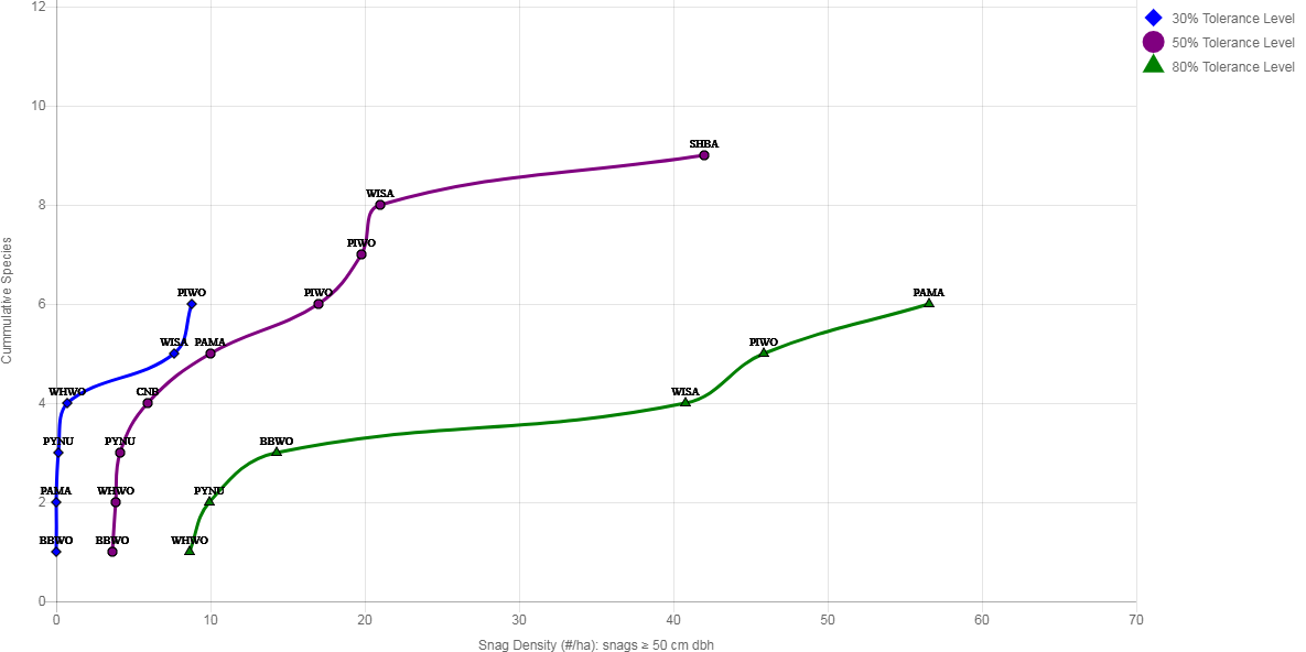
Figure 2 is an example from one vegetation condition in DecAID. Note the cumulative species curves look at an array of species using this habitat. Using the parameter of large snag density (snags > 20 inches dbh) at pileated woodpecker nest sites from the Eastside Mixed Conifer Forest, Late (EMC_L) wildlife habitat type we can say that in the EMC_L vegetation condition (you can also hover over the species code and get the density):
- 30% tolerance level = 3.5 large snags/acre (8.8 snags/ha), thus, 30% of nest sites used by pileated woodpeckers have < 3.5 large snags/acre and 70% of nest sites used by pileated woodpeckers have > 3.5 large snags/acre
- 50% tolerance level = 7.8 large snags/acre (19.4 snags/ha), thus, 50% of nest sites used by pileated woodpeckers have < 7.8 large snags/acre and 50% of nest sites used by pileated woodpeckers have > 7.8 large snags/acre
- 80% tolerance level = 18.4 large snags/acre (45.9 snags/ha), thus, 80% of nest sites used by pileated woodpeckers have < 18.4 large snags/acre and 20% of nest sites used by pileated woodpeckers have > 18.4 large snags/acre
Figure 2. Cumulative species curves for density (#/ha) of snags > approximately 25 cm dbh: species use of areas for nesting and roosting with documented snag densities for 30%, 50%, and 80% tolerance levels in the Eastside Mixed Conifer Forest Wildlife Habitat Types and Late Successional Structural Class.
The bottom line: The higher the tolerance level, the higher the proportion of individuals in the population that are being provided for, and the more assurance you have that you are providing habitat that will meet the needs of more individuals in the population. The basic assumption is that more is better and bigger is better. There are a few exceptions (e.g., black-backed woodpecker and Lewis' woodpecker which are noted in the Summary Narratives (yet another reason to read the Summary Narratives)).
Technicalities aside, what this all means in this example is that the higher the snag density (or the higher the tolerance level) the more likely that a pileated woodpecker will use the site and thus the more likely you are providing suitable habitat for the species.
Inventory data
The inventory tolerance levels are calculated also at 30%, 50%, and 80%. This makes the inventory data directly comparable to the wildlife data. However, the inventory tolerance levels were calculated differently, because these data are highly skewed to the left (Figure 3). This is because areas with lower amounts of dead wood are much more common on the landscape than areas with very high amounts of dead wood. See the Statistical Basis Paper for details on how tolerance levels were calculated.
Figure 3. Example distribution of snag densities from inventory plots by tolerance interval
For inventory tolerance levels, the "population" is the number of acres in the Vegetation Condition Class that the plots sampled. The tolerance level is then just the percentage of the landscape (not the same as the percentage of the sample plots) meeting the specified condition. For example, the 80% tolerance level for snag density is 19.7 snags/acre >10 inches dbh in the Eastside Mixed Conifer, East Cascades/Blue Mountains, Mid Successional Structure Class (EMC_ECB_M), the interpretation would be that 80% of the area in EMC_ECB_M would have snag densities of < 21.7 snags/acre, and 20% of the area would have snag densities > 19.7 snags/acre.
An important note: It is important to keep in mind that the vegetation inventory data came from plots of 1 ha or less, so the 20% of the area with > 19.7 snags/acre is likely distributed in high density clumps, and the plots with zero snags probably sampled low-density gaps. Thus you would not expect a whole stand to average > 1937 snag/acre unless the stand had experience above average mortality.
Tolerance levels for the inventory data from unharvested plots are displayed in 2 ways within the tables beneath the cumulative species curves: 1) only plots with measurable snags or down wood and 2) all unharvested plots regardless of whether they contained measurable snags or down wood. Each type has an appropriate use.
- Tolerance levels for vegetation plots with measurable snags or down wood should be applied in concert with the wildlife data. The assumption is that by definition dead wood dependent wildlife won't use that portion of the landscape without dead wood. Much of the wildlife use data were collected in plots associated with some type of use of dead wood (e.g., nesting, roosting, or foraging activities). If management of habitat for dead wood dependent species is a high priority on the project, these would be the tolerance levels to use.
- Tolerance levels for vegetation plots with and without measurable snags or down wood should be used in concert with the inventory distribution histograms. These tolerance levels incorporate the entire landscape including the portion with no measurable dead wood. These would be the tolerance levels to use if trying to use DecAID inventory data as a reference condition.
Comparing cumulative species curves to tolerance levels from vegetation inventory data will clearly demonstrate if wildlife species are using that portion of the landscape with high density clumps of dead wood; the wildlife tolerance levels will be considerably higher than the tolerance levels from inventory plots.
For more information on tolerance levels, see the sections of DecAID listed in Table 2.
Table 2. Documents in DecAID that provide information on tolerance levels.
| DecAID Document | Document contents |
|---|---|
| What is DecAID? | Takes you through the steps of running a DecAID query. Also explains how to interpret wildlife species curves and vegetation inventory summaries. Includes a brief description of tolerance levels. |
| What is a tolerance level? | A less technical, though detailed, description of tolerance levels. Compares tolerance levels to the more commonly used confidence intervals. |
| Marcot et al. 2010 | A published manuscript on the use of tolerance levels in DecAID. Relatively technical. Read this if you want all the details. |
Use the Appropriate Scale
The vegetation inventory data in DecAID from the unharvested portion of the landscape can be used as a reference condition; it is a coarse-filter approach to management at a broad landscape scale. The recommendation in DecAID for the size of the broad landscape is: "It is impossible to specify a single minimum size [analysis] area that is most appropriate to all ecoregions and geographic areas. However, as a general rule-of-thumb we suggest that [analysis] areas be at least 20 square miles in size [12,800 acres]." DecAID also states: "Analysis areas (landscapes or watersheds) should be sufficiently large to encompass the range of variation in wildlife habitat types and structural conditions that occur in the area." Obvious violations of this assumption need to be addressed, usually by increasing the size of the analysis area to incorporate the full variation within habitats. A common example is the case of large fires or insect outbreaks. At a watershed scale it may appear that there is an excess of dead wood because many disturbances are as large, or larger, than the watershed scale. But, it may still be a rare occurrence at the regional or sub-regional scale, the scale at which the vegetation data were collected. See the Determining Size of Analysis Area document for how to deal with this situation.
If a landscape level analysis has not been completed, then the vegetation distribution data should not be used to set management goals for dead wood habitat. Wildlife data were collected at a plot scale and thus can be used at a finer or fine-filter scale. Depending on the objectives of the land allocations which overlay the project, and the capability of the site, determine the appropriate level of habitat (i.e., tolerance level) that should be provided for dead wood dependent species on different parts of the landscape.
In general, the larger the analysis area, the more flexibility the manager has with managing dead wood in the project area. Other areas of the broader landscape may be providing quality dead wood habitat, and thus the onus for providing high levels of dead wood may not need to fall on the individual project.
Ideally, dead wood analysis and objectives for management of dead wood would be done once for each forest. This scale more accurately reflects the range of habitat types and structure stages represented by the inventory data. All the available data and GIS layers could be brought together and assessed in one fell swoop, saving time and money when compared to a piece-meal, project-by-project approach. An obvious opportunity for this assessment would be during Forest Plan Revision. Most revisions are still many years away, however, so forests may want to conduct the dead wood analysis independently of the revision process.
A regional-scale analysis was completed in October 2014 for all of Region 6. Using ArcGIS, the outputs from the analysis can be clipped to the forest or watershed and used as is, or can be modified with local data. See Region-wide Distribution Analysis under Links to Usefull Information.
Using Distribution Histograms as Reference Conditions
The terms Historic Range of Variability (HRV), Natural Conditions, and Historical Conditions are sometimes used interchangeably to indicate conditions which occurred on the landscape prior to the influence of humans (particularly Europeans). Because it is difficult to determine what snag and down wood levels were prior to influence of humans, the term "reference condition" is used in this document in terms of the use of inventory data from DecAID. While the data may not precisely reflect pre-European levels, the data do provide a reference condition for managers. See the HRV Dead Wood Comparison document for more information.
Data from unharvested plots can be used as a reference condition to approximate HRV of dead wood. By managing habitat within HRV it is assumed that adequate habitat will be provided because species survived those levels of habitat in the past to be present today. The further current conditions deviate from HRV the less likely adequate habitat is being provided to sustain those species using the habitat.
However, there is a caveat to using this approach in eastside dry forests:
On the eastside in particular, current levels of dead wood may be elevated above historical conditions due to fire exclusion and increased mortality, but may also be depleted below historical levels in local areas burned by intense fire or subjected to repeated salvage and/or firewood cutting. Conversely, plot data from unharvested forests on the westside when fire return intervals are longer, may provide a reasonable approximation of historical conditions.
There is debate among professionals on the impact fire exclusion has on stands relative to HRV. Thus, DecAID also presents information in the summary narratives from research studies and inventories about HRV where available. This additional information can be used to assess appropriateness of using data from unharvested plots to determine reference conditions, and to help identify knowledge gaps and areas of needed research.
Even with the caveats associated with applying inventory data to eastside forests to represent HRV, this guide still recommends using the data because:
- They are still some of the best data available to assess HRV of dead wood, even in eastside dry forests.
- They are the only available data showing distribution and variation in snag and down wood amounts across the landscape.
- The data from unharvested stands are in the range of other published data on HRV of dead wood even in the drier vegetation types. For a full discussion see HRV Dead Wood Comparison.
Snag densities and down wood percent cover are often higher at sites used by wildlife than would be indicated by the use of inventory data alone. Wildlife species may be selecting for clumps of snags around nest sites, dens, etc. which are areas represented by the wildlife species data. Information on reference conditions should usually be supplemented with an analysis of wildlife habitat as outlined in the Wildlife Tolerance Analysis for Green Projects or the Wildlife Tolerance Analysis for Salvage Sales analysis processes. This is particularly important in the Wildlife Habitat Types where a large portion of the landscape has 0 snags/acre (e.g., PPDF). Wisdom et al. (2000) state: "Source habitats for most species declined strongly from historical to current periods across large areas of the [Columbia] basin. Strongest declines were for species dependent on low-elevation, old-forest habitats (family 1)."Family 1 includes several cavity-nesting birds (Lewis' woodpecker, white-headed woodpecker, white-breasted nuthatch, pygmy nuthatch). Because of the concern over these species it may be prudent to manage more of the landscape in these low-elevation habitats for quality habitat (e.g., providing snags) than would be indicated by the information from the inventory distribution histograms.
Applying DecAID to Projects
DecAID is not management direction. Again remember it is just a compilation and interpretation of the best available science. However, this implementation guide is intended to give some suggestions and examples of how to use the data in DecAID to assess impacts of projects on dead wood and species that depend on dead wood.
There are a variety of projects that impact dead wood habitat. There is also more than one type of analysis that can be done for a project using data in DecAID to assess the impacts. Analysis can be fairly simple to complex. Keep in mind that the level of analysis needs to be concurrent with the complexity and risk of the proposed action.
Experience using DecAID for projects across the region has shown that a Distribution Analysis (see Tables 3 and 4) is a good way to address dead wood habitat in project planning and analysis. This analysis has been run for all Forest Service lands in Region 6 (Region-wide Distribution Analysis). The regional analysis can be easily used at the forest or watershed scale following the instructions provided with the data.
Remember, an analysis using DecAID is not a viability analysis. By using the information in DecAID the likelihood that adequate dead wood habitat is being provided can be assessed. A viability analysis will require an assessment of other factors that may be impacting the species populations. Information on populations from local data or other wildlife trend data sources (e.g., Breeding Bird Surveys) should be included in the assessment of viability. For eastside forests, the viability work completed by the ICBEMP project can be tiered to. A good source of information is the Source Habitats analysis and documents (see HRVTrend Data Sources under Links to Useful Information).
Below are 2 tables displaying the different types and levels of analysis presented in this guide; Table 3 for green sales and Table 4 for salvage sales after stand-replacing disturbances. Click on the analysis methods to see detailed description of the process and the examples to see how the method has been applied to actual projects. The project risk column refers to the risk of the project in terms of environmental consequences and/or likelihood of litigation. The other columns in the tables give brief information on application and intensity of data needed.
Caution: The examples in Tables 3 and 4 are the best examples of analysis using DecAID to date (i.e. NEPA process tried and tested with success). None of them are perfect. Some of them have some minor errors in wording and interpretation. Some do not adequately cite the appropriate table or figure from DecAID. For this reason, do not just adopt one of the examples and "cut and paste" your specific information in to the documents. In addition, the following examples are not the only way to utilize DecAID at the project level. Biologists are encouraged to explore new avenues for using DecAID. However, if you choose to do something drastically different than what is in this guide, it is recommended that a member of the DecAID Implementation Team be consulted to assure the information and data were used appropriately.
Sales in Green Tree Dominated Stands
One of the first questions people ask about green sales is: Why do we need to do a dead wood analysis for green projects where we are not cutting dead trees?? Good question! The answer is that thinning activities capture mortality and increase vigor of stands, thus impacting dead wood recruitment for decades especially if the stand is on a rotation. A dead wood analysis is beneficial in assessing the impact of harvest activities on dead wood, and setting objectives. For instance it may be that thinning sales are done to different prescriptions that will allow creation of snags following sale activities in watersheds depauperate of snags. Likewise it might call for thinning to wider spacing to more quickly grow larger green trees that can eventually become (larger) snags. For a good review of the "best available science" on thinning and dead wood see Thinning and Dead Wood: "Best Available Science".
For the purposes of this document, some salvage sales should be considered "green sales". If salvage is occurring primarily in stands that haven't undergone a stand-replacing disturbance, then the green sales approach is appropriate. Some examples would be removing hazard trees from along roads or in campgrounds, harvesting pockets of wind throw or bug kill within an otherwise green stand, HFRA projects, etc.
Table 3 below summarizes three types of analysis. Most projects should include use of both inventory data and wildlife data from DecAID (where available).
Table 3. Analysis methods for sales in green tree dominated stands.
| Analysis Method | Scale | Application | Project Risk | Example(s) |
|---|---|---|---|---|
| Distribution Analysis | Watershed or larger |
|
Moderate to High |
Silver Lake (uses DecAID ver 2.0) 2007 MTH Thin (uses DecAID ver 2.0) |
| Wildlife Tolerance Level Analysis | Watershed or larger |
|
Moderate to High | Westside Project (uses DecAID ver 2.0) |
Salvage Sales After Stand-Replacing Disturbances
Salvage sales usually warrant a relatively complex analysis for several reasons:
- Salvage has the potential to impact very important but rare (temporally and spatially) habitat.
- Stand-replacing disturbance events provide a unique opportunity to provide areas on the landscape with high amounts of dead wood that many species are associated with.
- Salvage sales are often controversial, with competing public opinion and science.
Recently burned forests support a diverse community of cavity-nesting birds, with stand-replacing fires resulting in large local increases in abundance of these species (Hutto 1995, Kotliar et al. 2002, Saab et al. 2004). Salvage logging impacts the number of snags and down logs available to wildlife in both the short term and the long term. We recommend that when using DecAID information to analyze post-fire habitats in Eastside mixed conifer or ponderosa pine habitat types, the user review Saab et al. (2002), Saab et al. (2007), Saab et al. (2009) and Saab et al. (2011) to further understand cavity nester use of post-fire stands.
It is imperative that the appropriate scale is chosen for assessment in salvage sales. The first step in your assessment will be determining the appropriate scale for the analysis area (see Determining Size of Analysis Area). Salvage projects are usually in areas which have undergone stand replacing disturbances such as fire or insect infestation. High snag densities resulting from these disturbances are temporary because snag densities decline rapidly as snags fall in the first decade or so after the disturbance. As a result, stands which have recently sustained a stand-replacing disturbance are not well represented in the inventory data in DecAID, even those from unharvested plots; they are a small proportion of the larger landscape at any one point in time. Current snag densities in a disturbed area would not be comparable to the distribution histograms or tolerance levels for inventory data in DecAID. Larger fires can skew the current conditions, even at the scale of a 10th field HUC, to the point that the analysis area is no longer representative of habitat conditions from which the inventory data were collected. Only those plots with the highest sampled snag densities could be expected to have come from plots experiencing recent stand-replacing disturbances. These plots may come from large scale disturbances like stand-replacing fire, or from smaller scale disturbances such as bug-kill or root rot.
Determine which analysis methods are appropriate for the project. Three types of analysis are presented with examples (Table 4). The user may want to complete the Quick Assessment prior to conducting the more detailed Distribution Analysis or Tolerance Level Analysis. Most projects (beyond the Quick Assessment) will use more than one method and should include use of both inventory data and wildlife data from DecAID (where available).
Table 4. Analysis methods for salvage projects occurring after stand-replacing events.
| Analysis Method | Scale | Application | Data intensity | Project Risk | Example(s) |
|---|---|---|---|---|---|
| Quick Assessment | Watershed or larger |
|
Low | Moderate to High | Sunflower Salvage (uses DecAID ver 2.2) |
| Distribution Analysis | Usually sub-basin or larger |
|
Moderate to High | Moderate to High |
Sunflower Salvage (uses DecAID ver 2.2) Tiller Whiskey Salvage (uses DecAID ver 2.2) |
| Wildlife Tolerance Level Analysis | Usually watershed or larger |
|
High | Moderate to high |
Links to Useful Information
DecAID Webinars:
There is a series of webinars available on the use of DecAID.
The DecAID Primer - an introduction and overview of DecAID
- Watch the presentation
- pdf of the Power Point presentation - DecAIDPrimer_2015.pdf
The DecAID Website - an overview of the website and how to navigate within the website
DecAID Distribution Analysis - how to conduct a distribution analysis using the Regional assessment
Tolerance Levels - a discussion on what a tolerance level is, how it is used in DecAID, and how to interpret the data in DecAID
- Watch the presentation
- pdf of the Power Point presentation -DecAID_ToleranceLevels_2015.pdf
DecAID Specific Tools:
Data Availability Summary by Species - An Excel spreadsheet indicating what information is available by species in DecAID. Users can filter by columns to query information by species, habitat or information type.
Convert volume per acre to percent cover for down wood - use the volume per acre to percent cover_DecAID.xlsx spreadsheet.
Convert between tons/acre and percent cover - currently for eastside habitats only - use the documented_dwd_conversion.xls spreadsheet.
Dead wood capability - A table that indicates the relative potential of a site to provide high, moderate and low amounts of dead wood based on fire regime, vegetation series/sub-series, and topographic position.
GIS tools/layers:
Region-wide Distribution Analysis -
A new version of the Gradient Nearest Neighbor (GNN) data was released in 2014. The GNN data are up to date through 2012. A distribution analysis has been run for all of Region 6 using the 2012 GNN data. The data have been updated for large fires (>1,000 acres) through 2015 using RAVG maps (http://www.fs.fed.us/postfirevegcondition/index.shtml). See the DecAID Metadata for a list of fires included in the regional analysis. These data can be used as is and clipped to your forest boundary or watershed.
See the DecAID_Metadata spreadsheet in the “Documentation_info” folder for details about the data used in the analysis and the output data available.
The “Documentation_info” folder contains the DecAID metadata, instruction documents, and Excel templates for summarizing the Regional Analysis data and creating distribution histograms. The information is located at: T:\FS\Reference\GeoTool\r06\Toolbox\DecAID\Documentation_info OR Region-wide Distribution Analysis
The data used to run the Regional Analysis are available at: T:\FS\Reference\GeoTool\r06\Toolbox\DecAID\DecAID_data2012 OR Download here: DecAIDData2012
You will only need to use these datasets if you want to re-run the analysis. The mains reason to rerun the analysis would be to change dead wood amounts due to small fires or bug kill that has occurred since 2012 or large fires beyond 2015. You will also need to update the data if you want to use your local PVT or roads layers.
For those who prefer to run the analysis with local data instead of regional data, an Arc Toolbox is available at: T:\FS\Reference\GeoTool\r06\Toolbox\DecAID\R6_DecAIDTbox_huc10.tbx OR Download here: DecAID Tools
For updating data from RAVG map ArcGIS Tool - An ArcGIS script is available to update the DecAID data for fires not included in the most recent RAVG update (currently most fires >1,000 acres through 2015). The tool can be downloaded from T:\FS\Reference\GeoTool\r06\Toolbox\DecAID\RAVG_Analysis OR Download here: RAVG Update
The output data from the Regional Analysis are located at: T:\FS\Reference\GeoTool\r06\Toolbox\DecAID\Output_data\R6 OR Download here: DecAIDRegionalOutputData
GNN Analysis Information -
Gradient Nearest Neighbor (GNN) vegetation maps - These maps are already available for several areas. In most cases, these maps contain actual detailed snag and down wood data at the pixel. See the following website for available data: http://www.fsl.orst.edu/lemma/main.php?project=imap&id=home . Also see Ohmann and Gregory (2002) for a discussion of the GNN approach.
The latest version of the GNN data is from 2012. These are the data used in the Region-wide Distribution Analysis.
Forest Insect and Disease Maps -
Information on insect- and disease-caused tree mortality as determined by aerial surveys is available at the following website: http://www.fs.fed.us/r6/nr/fid/data.shtml. Aerial survey flights are conducted each year and maps estimated numbers of trees killed by causal agent are available on the website. Each year, only the new mortality is mapped, so to get estimates of cumulative mortality over a period of time, data from all years within the time period must be added together. Preliminary data from recent projects have shown that these maps tend to consistently underestimate snag densities. In areas where there has been significant amounts of recent insect-caused mortality, this may be sufficient information to determine that snags levels meet or exceed the desired levels. Where mortality levels are not sufficient to make this call, these maps can be used to stratify the landscape when designing snag surveys across the landscape as per Bate et al. (2008).
Contact Ben Smith (bsmith02@fs.fed.us)(WA), Bob Schroeter (rschroeter@fs.fed.us)(OR), or Zach Heath (zheath@fs.fed.us) for assistance in interpreting the data appropriately.
Wildfire Maps and Tools:
BAER Fire Severity Map - fire severity maps from the Remote Sensing Application Center (RSAC) immediately post fire: http://www.fs.fed.us/eng/rsac/baer/
RAVG (Rapid Assessment of Vegetation Condition after Wildfire) – 30-45 days following containment of a wildfire that burnt 1,000 acres or more of forested NFS land: http://www.fs.fed.us/postfirevegcondition/whatis.shtml. Download maps for a particular fire by running a query at the bottom of http://www.fs.fed.us/postfirevegcondition/index.shtml. It is suggested that the 4-Class RAVG map is used in a DecAID analysis (fire ID_rdnbr_ba4.tif).
MTBS (Monitoring Trends in Burn Severity)– only complete through 2012, but can request data 2 to 3 months after containment: http://www.mtbs.gov/index.html
Plant Associations:
Plant associations and plant association groups (PAGs) are classifications of potential vegetation and can be crosswalked to wildlife habitat types in DecAID. Most forests have plant association maps available. Visit http://ecoshare.info/products/gis-data/ or contact your local vegetation ecologist.
Survey techniques:
Bate, L.J.; Torgersen, T.R.; Wisdom, M.J.; Garton, E.O.; Clabough, S.C. 2008. SnagPRO: Snag and tree sampling and analysis methods for wildlife. Gen. Tech. Rep. PNW-780. Portland, OR: U.S. Department of Agriculture, Forest Service, Pacific Northwest Research Station. 80 p. http://www.fs.fed.us/pnw/pubs/pnw_gtr780.pdf
Bate, L.J.; Torgersen, T.R.; Wisdom, M.J.; Garton, E.O.; Clabough, S.C. 2008. Log sampling methods and software for stand and landscape analyses. Gen. Tech. Rep. PNW-746. Portland, OR: U.S. Department of Agriculture, Forest Service, Pacific Northwest Research Station. 93 p. http://www.fs.fed.us/pnw/pubs/pnw_gtr746.pdf
Wildlife Trend Data Sources:
USGS North American Breeding Bird Survey (BBS)
http://www.mbr-pwrc.usgs.gov/bbs/bbs.html
Partners in Flight - Species Assessment Database - global and regional trends and threats
http://www.rmbo.org/pif/pifdb.html
NatureServe - State and Global Ranks
http://www.natureserve.org/explorer/
HRV Trend Data Sources:
The Source Habitats GTR contains information on habitat trends and is the basis for the viability assessment for the ICBEMP. It can be tiered to in viability assessments for projects.
The GTR is a 3-volume set. Volume 1 contains habitat trends for families as well as issues and strategies for dealing with the issues. In volume 1, Table 7 provides an assessment for individual species and gives a rank of -2 to 2. Those species with a rank of -2 are of special concern, those with a -1 also still warrant some concern. Table 12 summarizes trends by Ecological Reporting Unit (ERU) which allows you to see the situation in your particular geographic area. The last part of volume 1 discusses road-related issues. Volume 2 provides the same discussion at the finer group level. Sections on Interpreting Results and Management Implications are provided. Volume 3 contains the appendices. Table 3 gives habitat trends by ERU, providing information on your particular geographic area.
Wisdom, Michael J., Richard S. Holthausen, Barbara C. Wales, Christina D. Hargis, Victoria A. Saab, Danny C. Lee, Wendel J. Hann, Terrell D. Rich, Mary M. Rowland, Wally J. Murphy, and Michelle R. Eames. 2000. Source Habitats for Terrestrial Vertebrates of Focus in the Interior Columbia Basin: Broad-Scale Trends and Management Implications. General Technical Report PNW-GTR-485, Portland, OR. http://www.fs.fed.us/pnw/pubs/gtr485/
The work of Wisdom et al. (2000) was further assessed and was published in Forest Ecology and Management:
Raphael, M.G., M.J. Wisdom, M.M. Rowland, R.S. Holthausen, B.C. Wales, B.G. Marcot, and T.D. Rich. 2001. Status and trends of habitats of terrestrial vertebrates in relation to land management in the Interior Columbia River Basin. Forest Ecology and Management 153:63-88.
DecAID Implementation Team
| Name | Location | Phone | |
|---|---|---|---|
| Barbara Garcia, Regional Wildlife Ecologist | Regional Office, Pacific Northwest Region | 503-808-2993 | bagarcia@fs.fed.us |
| Barbara Webb, DecAID Center of Excellence | Bend-Fort Rock RD, Deschutes NF | 541-383-4788 | bswebb@fs.fed.us |
| Steve Acker | NW Oregon Ecology Program | 541-225-6447 | stevenaacker@fs.fed.us |
Literature Cited
Bate, L.J.; Torgersen, T.R.; Wisdom, M.J.; Garton, E.O.; Clabough, S.C. 2008. SnagPRO: Snag and tree sampling and analysis methods for wildlife. Gen. Tech. Rep. PNW-780. Portland, OR: U.S. Department of Agriculture, Forest Service, Pacific Northwest Research Station. 80 p. http://www.fs.fed.us/pnw/pubs/pnw_gtr780.pdf
Bate, L.J.; Torgersen, T.R.; Wisdom, M.J.; Garton, E.O.; Clabough, S.C. 2008. Log sampling methods and software for stand and landscape analyses. Gen. Tech. Rep. PNW-746. Portland, OR: U.S. Department of Agriculture, Forest Service, Pacific Northwest Research Station. 93 p. http://www.fs.fed.us/pnw/pubs/pnw_gtr746.pdf
Chappell, Christopher B., Rex C. Crawford, Charley Barrett, Jimmy Kagan, David H. Johnson, Mikel O'Mealy, Greg A. Green, Howard L. Ferguson, W. Daniel Edge, Eva L. Greda, and Thomas A. O'Neil. 2001. Wildlife habitats: Descriptions, status, trends, and system dynamics. Pp. 22-114 in: D.H. Johnson and T. A. O'Neil, ed. Wildlife-habitat relationships in Oregon and Washington. Oregon State University Press, Corvallis OR.
Harrod, Richy J., William L. Gaines, William E. Hartl, and Ann Camp. 1998. Estimating historical snag densities in dry forests east of the Cascade Range. USDA Forest Service, Pacific Northwest Research Station, Gen. Tech. Rept. PNW-GTR-428, Portland, OR. 16 p. http://www.fs.fed.us/pnw/pubs/gtr_428.pdf
Hutto, Richard. 1995. Composition of bird communities following stand-replacing fires in the northern Rocky Mountain (U.S.A.) Conifer Forests. Conservation Biology 9(5):1041-1058.
Kotliar, Natasha B., Sallie J. Hejl, Richard L. Hutto, Victoria A. Saab, Cynthia P. Melcher, and Mary E. McFadzen. 2002. Effects of fire and post-fire salvage logging on avian communities in conifer-dominated forests of the western United States. Studies in Avian Biology 25:49-64.
Marcot, B. G. 1992. Snag Recruitment Simulator, Rel. 3.1 [computer program], USDA Forest Service, Pacific Northwest Region, Portland OR.
Marcot, Bruce G., Janet L. Ohmann, Kim Mellen-McLean, and Karen Waddell. 2010. Synthesis of regional wildlife and vegetation field studies to guide managment of standing and down dead trees. Forest Sceince 56(4):391-404. http://www.fs.fed.us/r6/nr/wildlife/decaid/documents/marcot_etal_2010_DecAID.pdf
Mellen-McLean, Kim, Bruce G. Marcot, Janet L. Ohmann, Karen Waddell, Susan A. Livingston, Elizabeth A. Willhite, Bruce B. Hostetler, Catherine Ogden, and Tina Dreisbach. 2012. DecAID, the decayed wood advisor for managing snags, partially dead trees, and down wood for biodiversity in forests of Washington and Oregon. Version 2.20. USDA Forest Service, Pacific Northwest Region and Pacific Northwest Research Station; USDI Fish and Wildlife Service, Oregon State Office; Portland, Oregon. http://www.fs.fed.us/r6/nr/wildlife/decaid/
Neitro, W.A., V.W. Binkley, S.P. Cline, R.W. Mannan, B. G. Marcot, D. Taylor, and F. F. Wagner. 1985. Snags (wildlife trees). Pages 129-169 in E.R. Brown, technical editor. Management of wildlife and fish habitats in forests of western Oregon and Washington. USDA Forest Service, Pacific Northwest Region, Portland, OR. Publication No. R6-F&WL-192-1985.
Ohmann, J.L., and M.J. Gregory. 2002. Predictive mapping of forest composition and structure with direct gradient analysis and nearest neighbor imputation in coastal Oregon, USA. Canadian Journal of Forest Research: 32:725-741. http://www.fsl.orst.edu/lemma/common/export/pubs/ohmann_gregory_2002_CJFR.pdf
Raphael, M.G., M.J. Wisdom, M.M. Rowland, R.S. Holthausen, B.C. Wales, B.G. Marcot, and T.D. Rich. 2001. Status and trends of habitats of terrestrial vertebrates in relation to land management in the Interior Columbia River Basin. Forest Ecology and Management 153:63-88.
Raphael, M. G. 1983. Cavity-nesting bird response to declining snags on a burned forest: a simulation model. (pp. 211-215) In: J. W. Davis, G. A. Goodwin, and R. A. Ockenfels (Ed.). Snag habitat management: proceedings of the symposium. USDA Forest Service General Technical Report RM-99. Flagstaff AZ.
Rose, C. L., B. G. Marcot, T. K. Mellen, J. L. Ohmann, K. L. Waddell, D.L. Lindley, and B. Schreiber. 2001. Decaying wood in Pacific Northwest forests: concepts and tools for habitat management. Pp. 580-623 in: D.H. Johnson and T. A. O'Neil, ed. Wildlife-habitat relationships in Oregon and Washington. Oregon State University Press, Corvallis OR. http://www.fs.fed.us/r6/nr/wildlife/decaid/pages/documents/Rose-et-al-2001.pdf
Saab, Victoria A., Robin E. Russell, Jay Rotella, Jonathan G. Dudley. 2011. Modeling nest survival of cavity-nesting birds in relation to postfire salvage logging. Journal of Wildlife Management 75(4):794-804. http://www.treesearch.fs.fed.us/pubs/38683
Saab, Victoria A., Robin E. Russell, Jonathan G. Dudley. 2009. Nest-site selection by cavity-nesting birds in relation to postfire salvage logging. Forest Ecology and Management 257:151-159. http://www.treesearch.fs.fed.us/pubs/31757 and updated Appendix A
Saab, Victoria A., Robin E. Russell, and Jonathan G. Dudley. 2007. Nest densities of cavity-nesting birds in relation to postfire salvage logging and time since wildfire. Condor 109:97-108. http://www.treesearch.fs.fed.us/pubs/27685
Saab, Victoria A., Jonathan Dudley, and William L. Thompson. 2004. Factors influencing occupancy of nest cavities in recently burned forests. Condor 106:20-36.
Saab, V., R. Brannon, J. Dudley, L. Donohoo, D. Vanderzanden, V. Johnson, and H. Lachowski. 2002. Selection of fire-created snags at two spatial scales by cavity-nesting birds. In: Laudenslayer, William F., Jr.; Valentine, Brad; Weatherspoon, C. Philip; Lisle, Thomas E., technical coordinators. Proceedings of the symposium on the ecology and management of dead wood in western forests. 1999 November 2-4; Reno, NV. Gen. Tech. Rep. PSW-GTR-181. Albany, CA: Pacific Southwest Research Station, Forest Service, U.S. Department of Agriculture. http://www.fs.fed.us/psw/publications/documents/gtr-181/062_Saab.pdf
Thomas, J. W., R. G. Anderson, C. Maser, and E. L. Bull. 1979. Snags. Pp. 60-77 in: J. W. Thomas, ed. Wildlife habitats in managed forests the Blue Mountains of Oregon and Washington. Agriculture Handbook No. 553. USDA Forest Service, Portland OR.
Wisdom, Michael J., Richard S. Holthausen, Barbara C. Wales, Christina D. Hargis, Victoria A. Saab, Danny C. Lee, Wendel J. Hann, Terrell D. Rich, Mary M. Rowland, Wally J. Murphy, and Michelle R. Eames. 2000. Source Habitats for Terrestrial Vertebrates of Focus in the Interior Columbia Basin: Broad-Scale Trends and Management Implications. General Technical Report PNW-GTR-485, Portland, OR. http://www.fs.fed.us/pnw/pubs/gtr485/