DecAID Implementation: Green Tree Sales
Distribution Analysis for Green Projects
Objective of a Distribution Analysis
A distribution analysis allows you to compare current condition to reference conditions of amounts and distribution of dead wood across the landscape, as represented by the vegetation inventory distribution histograms in DecAID. The closer the current conditions are to reference conditions the higher the likelihood that adequate habitat is being provided for dead wood associated species and processes. This analysis can be conducted for snags or for down wood.
Project Area vs Analysis Area
Project areas are usually delineated to encompass an area containing stands to be treated. These areas are usually too small to adequately analyze the impacts of the project on dead wood levels across the landscape. The inventory data in the DecAID Advisor are appropriately used to assess dead wood at the landscape level, usually not at the project or stand scale.
The DecAID Advisor contains the following discussion on appropriate scale of application of the inventory data contained in the advisor:
"...it is reasonable to apply distributional information about dead wood that is based on many inventory plots in a given vegetation condition to a management "unit" at the scale of a landscape or sub-watershed. DecAID will be best applied at scales of subwatersheds, watersheds, subbasins, physiographic provinces, or large administrative units such as Ranger Districts, National Forests, or BLM Districts."
"When using the inventory data, analysis areas (landscapes or watersheds) should be sufficiently large to encompass the range of variation in wildlife habitat types and structural conditions that occur in the area in which the inventory data were collected (i.e. representative of variation at the sub-regional scale). It is impossible to specify a single minimum size analysis area that is most appropriate to all ecoregions and geographic areas. However, as a general rule-of-thumb we suggest that analysis areas be at least 20 square miles (12,800 acres, 5,120 ha) in size. This coincides with the small end of the range of sizes typical of 10th-field hydrologic unit codes (HUCs). The exception would be when managing habitats that are rare at a broad geographic scale, even if they are common at the watershed scale (e.g. recent post-fire habitats). Even at the scale of the 10th-field HUC, wildlife and inventory summaries for multiple vegetation conditions will need to be considered in the analysis and planning process."
Snag and down wood levels in the analysis area can be compared against the information from inventory data contained in DecAID only if the area is large enough to allow such a comparison. The analysis area should be large enough to represent the variation in snag habitat and distribution from which the inventory data were collected. If this is not possible, a comparison between the project area and the inventory data may not be appropriate.
Based on the above discussion, a minimum analysis area would include all those 10th field hydrologic units (watersheds) or 12th field hydrologic units (subwatersheds) intersected by the analysis area, if it totals at least 20 square miles (12,800 acres). This is the minimum size for each Wildlife Habitat Type. An analysis area of this size allows a comparison between current conditions and the vegetation inventory distribution histograms. This "rule-of-thumb" should apply to most projects in green forests (i.e. regeneration harvest, commercial thinning, etc.).
Region-wide Distribution Analysis
Steps 1-4 of a distribution analysis, as described below, have been run for all Forest Service lands in Region 6 using the 2012 GNN data (and updated as the GNN is updated). These data can be used as is and clipped to your forest boundary or watershed.
The region-wide analysis is available with or without buffering for roads. For the outputs with buffering for roads, snag densities were reduced by 40% within 50 meters of roads to account for falling of hazard trees, firewood cutting, etc., as per Bate et al. (2007), and Wisdom and Bate (2008). Determining which layer to use will depend on the extent of firewood cutting along roads in your area.
The user will still need to:
- identify the Wildlife Habitat Types in the analysis area as described in Step 2.
- determine the HRV% for each Successional Structure Class as described in Step 3.
- complete steps 5 and 6.
To use this analysis follow the instruction documents in the following order:
Instructions for DecAID Regional Analysis, summary template, and distribution analysis template
To access the analysis go to the Region-wide Distribution Analysis section of the Links to Useful Information section on the main page of this web site.
A webinar has been developed to demonstrate the use of the Region-wide Distribution Analysis.
Distribution Analysis
Below is one method on how to perform a distribution analysis for a project. A snag analysis is outlined; a down wood analysis would follow the same steps.
Step 1:Data Collection: Determine current snag and down wood distribution across the landscape
This step has been completed for the entire region in the Region-wide Distribution Analysis. The region-wide analysis used GNN data circa 2012. The data have been updated for large fires (>1,000 acres) through 2014 using RAVG maps (http://www.fs.fed.us/postfirevegcondition/index.shtml). See the DecAID Metadata for a list of fires included in the regional analysis. If other disturbances or treatments have occurred in the analysis area since 2012, the dead wood data should be updated prior to conducting a Distribution Analysis. The following are examples of the types of disturbances and treatments that have not been incorporated into the Region-wide Distribution Analysis:
- Disturbances:
- Fires occuring in 2015 and beyond
- Insect and disease activity since 2012
- Past fires not included on RAVG maps (usually <1,000 acres)
- Treatments since 2012
- Salvage sales
- Hazard/danger tree treatments
- Fuels reduction treatments
Supplemental data may need to be used to update the data for disturbances or activities that have occurred since 2012. Here are some examples of survey methods or data that may be available:
- Ground surveys - A good methodology can be found in Bate et al. 1999 http://www.fs.fed.us/pnw/pubs/gtr_425.pdf
- Recent stand exams (caveat - on some forests only merchantable snags were measured, and not all stands have stand exams - they also may not represent a systematic sample of overall conditions).
- FVS - FVS (Forest Vegetation Simulator) can run old stand exam data to project current snag levels. Normalizes data from stand exams taken in different years and puts them into one year.
- GIS mapping of various forest stands based on past management can be used to modify snag and down wood densities as needed. Some examples of possible categories are:
- Data for recent treatments from project implementation can be found in your local FACTS database.
- Roads have been buffered in the Region-wide Distribution Analysis using a regional roads layer. A local roads layer could be used to more accurately buffer roads. For those who prefer to run the analysis with local data instead of regional data, an Arc Toolbox is available at: T:\FS\Reference\GeoTool\r06\Toolbox\DecAID\R6_DecAIDTbox_huc10.tbx OR Download here: DecAID Tools
- Developed recreation sites, administrative sites, etc. where hazard tree removal has reduced snag levels based on the local Forest policy. This area can be determined by calculating the distance from each site. The resulting acreage can be assigned a snag density.
- Recent fires create varying densities of snags depending on fire intensity and severity. There are several sources for data on fires. See the Wildfire maps section of the Links to Useful Information section at the bottom of this page.
- Areas of high snag densities due to other disturbances (e.g. insect infestations where high mortality occurred, areas of root rot, etc.). Region 6 conducts annual aerial surveys of insect- and disease-caused mortality and most National Forests should have this information available in their GIS systems. If not, it can be downloaded from the RO Forest Health Protection website (Aerial Survey Data). These data can be used to help determine areas with high levels of mortality. Annual surveys only calculate "new" dead based on changes in foliage color, so there is a need to overlay multiple years of aerial data. Using 5 to 10 years of aerial data may better reflect existing conditions. If you need assistance in interpretation of the data or in converting data to cumulative numbers of dead trees per acre, contact Ben Smith (bsmith02@fs.fed.us)(WA), Bob Schroeter (rschroeter@fs.fed.us)(OR), or Zach Heath (zheath@fs.fed.us) for assistance in interpreting the data appropriately. Forest Service researchers have been field testing the accuracy of the aerial survey data and their preliminary conclusions suggest that surveys underestimate snag levels. At this time, a general "rule of thumb" is to multiply the reported values by 3.
Step 2:Determine Wildlife Habitat Types (WHTs) in the Analysis Area
Links to descriptions and maps of the inventory plots are provided on the DecAID query page to assist the user in determination of the Wildlife Habitat Type(s) for a project area. There may be situations where the habitat type(s) in an analysis area are difficult to determine. In such cases, or wherever there is uncertainty about the Wildlife Habitat Type, you should consult the Summary Narratives in DecAID under Habitat Type Descriptions section. More detailed descriptions are provided by clicking on the View Maps link on the top toolbar. Each map gives descriptions, maps, and pictures of the Wildlife Habitat Type
Descriptions of the habitat types and vegetative composition information for the possible Wildlife Habitat Types in your area can be compared allowing one to select the type that is the closest match. There may be more than one Wildlife Habitat Type in an analysis area. Each should be identified.
The Region-wide Distribution Analysis uses Potential Vegetation Types (PVTs) from the Integrated Landscape Assessment Project (ILAP), cross-walked to DecAID Wildlife Habitat Types. If these PVTs are a poor fit for your area, your local PVT map can be used. However, this will require re-running the distribution analysis using the new PVT map. For those who prefer to run the analysis with local data instead of regional data, an Arc Toolbox is available at: T:\FS\Reference\GeoTool\r06\Toolbox\DecAID\R6_DecAIDTbox_huc10.tbx OR Download here: DecAID Tools
Step 3:Determine Historical Structural Condition(s) Within Each Wildlife Habitat Type in the Analysis Area
The minimum analysis area for applying the inventory data from DecAID is approximately 12,800 acres per Vegetation Condition. At this scale, wildlife and inventory summaries for multiple Vegetation Conditions will need to be considered in the analysis and planning process. Remember, Vegetation Conditions in DecAID are a combination of Wildlife Habitat Type and Successional Stucture Class. There are likely multiple Successional Structure Classes in each Wildlife Habitat Type occurring in the analysis area. To avoid needing an analysis area large enough to encompass 12,800 acres of each Vegetation Condition, a weighted average across Structural Condition Classes can be calculated for each Wildlife Habitat Type to reduce the size of the analysis area. The weighted average is calculated in the HRV tabs of the Summary spreadsheets in the Region-wide Distribution Analysis.
Consult with a Silviculturist, reference available Watershed Analysis, etc. to estimate what percent of the landscape was within each structural class for each Wildlife Habitat Type historically. To do this, one must become familiar with how the structural classes are used and described in DecAID. Successional Structure Classes are described in the Summary Narratives of DecAID under the Structural Condition Description section. The "View Maps" tab on the top toolbar will take you to a "Successional Structure Class Description section with basic descriptions to assist the user in determination of the Successional Structure Class(es) present within each Wildlife Habitat Type.
Step 4:Build “Current Condition” Distribution Histograms for Each Wildlife Habitat Type and Compare to Vegetation Inventory Histograms
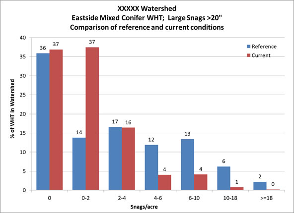
Distribution histograms are automatically created in the DecAID Distribution Analysis spreadsheets in the Region-wide Distribution Analysis. Histograms should to be created for each WHT in the Analysis Area, and for each dead wood type and size class (e.g., snags >25 cm and >50 cm; down wood >12.5 cm and >50 cm).
Figure 1. An example of a comparison of "reference" or "natural" conditions from the Region-wide Distribution Analysis for snags >20" dbh.
If you do not use the Regional Distribution Analysis complete the following:
Refer to the Distribution Histograms for a specific habitat type and determine the most appropriate way to break out the snag density ranges (e.g.*.inv-14 in DecAID). Be sure to convert the densities/hectare from DecAID to densities/acre. For example, snag distributions could be grouped by 0, 0-10, 10-20, 20-30, 30+ snags per acre. Determine what percentage of the landscape is in those various snag density categories by structural stage. Determine what the distribution is for the snag density categories for the structural stages that will be present within the analysis area. Develop a table that displays the percent of area within each snag density category for each structural stage needed for each vegetation type based on the distribution histograms
Step 5:Assess the effect of project on future snag habitat
Even if no snags are being harvested in the project, silvicultural treatments are likely to have an effect on the recruitment of snags in the future. This step can be either qualitative or quantitative depending on project risk and magnitude of anticipated effects.
A qualitative assessment would involve discussion of effects such as expected reduction or increase in mortality, and impact to size of future snags. For instance it may be that thinning sales will allow creation of snags following sale activities in watersheds depauperate of snags, but may also decrease risk of mortality due to suppression or insect and disease outbreaks and thus suppress snag creation for decades into the future. Thinning to wider spacing may more quickly grow larger green trees that can eventually become (larger) snags, but make sure to discuss the mortality mechanism that will turn the larger trees in to snags in the future. Prescribed burning may reduce dead wood habitat at least in the short term (Bagne et al. 2008).
A quantitative assessment is recommended for most projects and can be accomplished by running the Forest Vegetation Simulator Fire and Fuels Extension (FVS-FFE) with the assistance of your silviculturist or fuels planner. The analysis will show both future stand structure with associated mortality and dead wood dynamics including snag fall and decay. There are several ways to display the results of the analysis. A couple examples are displayed below.
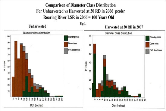
Notice, that for this particular site and treatment, there will be a few more large trees (green bars) and snags in most sizes (gray bars) in 60 years with treatment versus non-treatment. However, the impact to down trees less than about 16" in diameter is high.
Figure 3. An example of outputs from FVS-FFE that displays snag densities over 90 years, comparing a no action alternative to light and moderate thin alternatives.
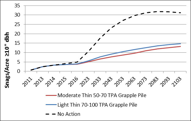
Notice, that for this particular site and treatments, there will be significantly fewer snags >10" dbh for at least 10 to 80 years post-treatment.
Step 6:Discuss "So What" Questions to the Distribution Analysis.
Example Questions
- Is the analysis area deficient in small or large snags?
- Is the analysis area deficient in a specific density of snags (ex. rare patches of high density snags)?
- What effects could this have on dead wood dependent species?
- Is there other data that can be referenced from DecAID (other than the vegetation inventory data) or other literature on historical snags densities or snag distribution? If so, use this information and compare it to current conditions.
- Is there other data to indicate the amount of landscape in a rare condition of having very high densities of snags (ex. historical post-fire mapping)? If so, use this information and compare it to current conditions. A recommended source is:
Harrington, Constance A., comp. 2003. The 1930s survey of forest resources in Washington and Oregon. Gen. Tech. Rep. PNW-GTR-584. Portland, OR: U.S.Department of Agriculture, Forest Service, Pacific Northwest Research Station. 123 p. [plus CD-ROM].
The distribution histograms in DecAID represent the best available estimate of "natural (unharvested) conditions" and thus reference conditions. Recognize that, particularly on the east side of the Region, fire control with missed fire intervals has resulted in conditions that may not be historical. For a full discussion see HRV Dead Wood Comparison.
Comparison of the "current situation" histograms with the DecAID histograms can help understand to what extent the analysis area provides snags and down wood, by comparing the range of tolerance levels shown in the histograms. If differences are evident between the current situation histogram and the DecAID reference conditions histogram, then objectives can be established to adjust snag or down wood size or abundance which will help move the landscape toward a condition which more closely resembles the reference conditions. If the project is not expected to move the landscape toward reference conditions due to competing issues (e.g. WUI, campground, hazard tree removal, etc.) a discussion of why this cannot be accomplished with this project should be provided. This discussion should also include a discussion of where on the larger landscape dead wood habitat will be provided.
Relationship to Wildlife Habitat
Snag densities and down wood percent cover in DecAID are often higher at sites used by wildlife than would be indicated by the use of inventory data alone. Wildlife species may be selecting for clumps of snags around nest sites, dens, etc. which are areas represented by the wildlife species data. The information from this analysis of dead wood distribution should usually be supplemented with an analysis of wildlife habitat as outlined in the Wildlife Tolerance Level Analysis for Green Projects analysis process. This is particularly important in the Wildlife Habitat Types where a large portion of the landscape has 0 snags/acre (e.g. PPDF). Wisdom et al. (2000) state: "Source habitats for most species declined strongly from historical to current periods across large areas of the [Columbia] basin. Strongest declines were for species dependent on low-elevation, old-forest habitats (family 1).". Family 1 includes several cavity-nesting birds (Lewis' woodpecker, white-headed woodpecker, white-breasted nuthatch, pygmy nuthatch). Because of the concern over these species it may be prudent to manage more of the landscape in these low-elevation habitats for quality habitat (e.g. providing snags) than would be indicated by the information from the inventory distribution histograms.
References
Bagne, Karen E., Kathryn L. Purcell, John T. Rotenberry. 2008. Prescribed fire, snag population dynamics, and avian nest site selection. Forest Ecology and Management 255:99-105.
Bate, Lisa J.; Garton, Edward O.; Wisdom, Michael J. 1999. Estimating snag and large tree densities and distributions on a landscape for wildlife management. Gen. Tech. Rep. PNW-GTR-425. Portland, OR: U.S. Department of Agriculture, Forest Service, Pacific Northwest Research Station. 76 p. http://www.fs.fed.us/pnw/pubs/gtr_425.pdf
Harrington, Constance A., comp. 2003. The 1930s survey of forest resources in Washington and Oregon. Gen. Tech. Rep. PNW-GTR-584. Portland, OR: U.S.Department of Agriculture, Forest Service, Pacific Northwest Research Station. 123 p.[plus CD-ROM].
Mellen-McLean, Kim, Bruce G. Marcot, Janet L. Ohmann, Karen Waddell, Susan A. Livingston, Elizabeth A. Willhite, Bruce B. Hostetler, Catherine Ogden, and Tina Dreisbach. 2012. DecAID, the decayed wood advisor for managing snags, partially dead trees, and down wood for biodiversity in forests of Washington and Oregon. Version 2.2. USDA Forest Service, Pacific Northwest Region and Pacific Northwest Research Station; USDI Fish and Wildlife Service, Oregon State Office; Portland, Oregon. http://www.fs.fed.us/r6/nr/wildlife/decaid/
Wisdom, Michael J., Richard S. Holthausen, Barbara C. Wales, Christina D. Hargis, Victoria A. Saab, Danny C. Lee, Wendel J. Hann, Terrell D. Rich, Mary M. Rowland, Wally J. Murphy, and Michelle R. Eames. 2000. Source Habitats for Terrestrial Vertebrates of Focus in the Interior Columbia Basin: Broad-Scale Trends and Management Implications. General Technical Report PNW-GTR-485, Portland, OR. http://www.fs.fed.us/pnw/pubs/gtr485/