How to Use DecAID: A Tutorial
Running a DecAID Query
Here is a step-by-step tutorial on running DecAID. You can follow along here as you actually run a query in DecAID, or just explore on your own and use this section to clarify questions or to help discover new functions. We will offer Tips to describe selected buttons, links, or information on each page.
OK, let's get started.
-
Click on the "Access DecAID" button.
Tip: Note that the home page has a set of drop down menu links on the top of the page. These should be self-explanatory. Feel free to explore at your leisure.
-
Next, select from the pull-down menus on the left-hand side the Habitat and the Structural Condition for which you want information. If you are uncertain as to which wildlife habitat type to select, you can select a map of forest inventory plot locations from the top tool bar menu “View Maps” menu and view plot locations to see if they occur in your geographic location of interest. You can also read descriptions about the habitat type, successional structure class, and see example photos of the habitat here by scrolling on this portion of the page/screen.
Tip: Note that we have further split two of the habitats (Eastside Mixed Conifer Forest, and Westside Lowland Conifer-Hardwood Forest) into several geographic subdivisions, because the wildlife and inventory data suggested significant differences in these subdivisions.
-
The Narrative page. This is the highest-level summary and synthesis of all the DecAID data and information for the habitat and structural condition (collectively "vegetation condition") you specified. On the left hand side click on “Summary Narrative” and it will drop down a Table of Contents of different sections
Yes, it is a lot of information here, but don't get daunted - it is well organized into introduction, methods, results, and summary sections. Each of these sections is described next.
Tip: If you need the bottom line fast, just page down to the first section "Synthesis and Recommendations." Other information in the narrative, and all the links from the Narrative to other screens, build upon this.
Explore the Narrative from the top down. It is arranged as follows:
Table of Contents - for the entire page. Click on any entry to quickly skip to that section.
Synthesis and Management Implications - all the sections summarized into numbers and guideposts on wildlife use of snags and down wood, inventory summaries of snag and down wood levels, and other information. We encourage you to consider this synthesis but we also invite you to "drill down" deeper into the text narrative and the underlying data and draw your own conclusions and recommendations from the base information. We don't want this to be a black box; we want you to be able to see and evaluate for yourself as much of the information and data underlying our synthesis and management implications as possible.
Introduction to Vegetation Condition, Introduction to Available Data - text describing the habitat type and structural condition you selected for the query as well as basic information on the types of studies, data, and statistical analysis to the extent available for wildlife and inventory data.
Integrated Summary of the Wildlife Data and Inventory Data From Unharvested Plots - summarizes the data on wildlife use of snags and down wood at three tolerance levels (more on this below), and discusses how to interpret the inventory data on snags and down wood from unharvested plots in terms of "natural conditions." Links go to figures and tables showing the data underlying the summaries.
Ancillary Information on Wildlife Species Use of Decayed Wood Elements - presents summaries of any available information from the literature on the relationship between wildlife use and tree height, tree species, tree morality condition, hollow live trees and snags, snag decay, tree top condition, down wood length, down wood species, hollow down wood, down wood decay, and other factors.
General Wildlife-Habitat Relations with Wood Decay Elements - - information was taken from general wildlife-habitat relationships databases and not necessarily from field studies per se. This is provided because the actual field studies, used above, often do not provide field data on all possible wildlife species found associated with wood decay elements in a given vegetation condition. We wanted some way to provide you with fuller lists of wildlife species that might be found for the vegetation condition you queried.
Landscape-level Distribution of Decayed Wood Elements - comparisons of current and "natural" (unharvested) conditions from the forest inventory data. This information may be useful for describing current (including harvested) conditions and "reference" or "natural" (including unharvested) conditions. Links here drill down into more details of the inventory data, discussed further below.
Relationships of Fungi to Decayed Wood Elements - a summary of what is known about fungi and decayed wood. A link in this section takes you to a more detailed narrative on this topic but one that generally pertains to all forest habitats, as habitat-specific data on fungi and wood decay relations were lacking.
Considerations for Stand Dynamics - a discussion of vegetation dynamics and effects of insects, pathogens, and fire on stand structure. Links provide further, detailed information on insect and pathogen species. Also included, is a summary of the role of fire in this vegetation condition.
Ecological Functions and Processes of Decayed Wood Elements - links to lists of wildlife species associated with decayed wood elements and associated key ecological functions, and a summary of ecosystem processes related to wood decay with a link to a longer narrative. The aim of this section is to broaden thinking and discussion about wood decay to recognize the important ways that wood decay elements support a variety of ecological roles of wildlife and for other dynamics of ecosystems.
-
There are lots of ways to explore information about wildlife use of snags, down wood, and other wood decay elements, and about forest inventory data, insects and pathogens, fungi, ecological roles of wildlife associated with wood decay elements, and other topics.
Let's look first at the underlying wildlife data on use of snags and down wood. Under the Data tab on the menu on the left-hand side of the page is another menu that provides:
- - "Snag DBH" (wildlife use of snag diameter),
- - "Down Wood Diameter" (wildlife use of down wood by diameter),
- - "Snag Density" (wildlife use of numbers of snags per unit area, e.g., snags/acre), and
- - "Down Wood % Cover" (wildlife use of down wood by percent of the forest floor covered by down wood).
Click on Data, then Snag Density
This will take you to a page that usually has two wildlife line graphs on the top and from two to six inventory data tables. Both display tolerance levels for the data - see “What is a Tolerance Level?". Note that in the Westside Lowlands Conifer-Hardwood Forest vegetation conditions, there are additional box plot graphs representing data from an old-growth forest study (Spies et al. 1988).
Note that, whereas the inventory data and the summary narrative are specific to a subregion for Westside Lowland Conifer-Hardwood Forest and Eastside Mixed Conifer Wildlife Habitat Types, the wildlife data are not specific to subregion. Thus, the "cumulative species curve" graphs may include data from all subregions within the wildlife habitat type.
The wildlife line graphs are "cumulative species curves." Here is how to interpret these graphs.
The cumulative wildlife species curves display the synthesized data from wildlife studies for individual species, or groups of species if the data were presented that way by the researchers. The x axis is the size or amount of the particular decayed wood element (snag dbh, down wood diameter, snag density, or down wood percent cover). The y axis is the number of species for which there are data, and the data points are arranged from lowest x axis value to highest x axis value as number of species on the y axis increases. Each point is the value from one or more studies for the 30%, 50% (mean) and 80% tolerance levels, linked together in curves.
If there were data from more than one study for a given species, we weighted the values by sample size before plotting them on the graph. If a variability estimate for the data was not available, or the sample size was less than 5, then we displayed only the means (50% tolerance levels) for that species. When this happened, there are more data points on the 50% curve than the 30% and 80% curves.
In the example snag density graph below, the 50% tolerance level, or the mean, curve contains 3 species.
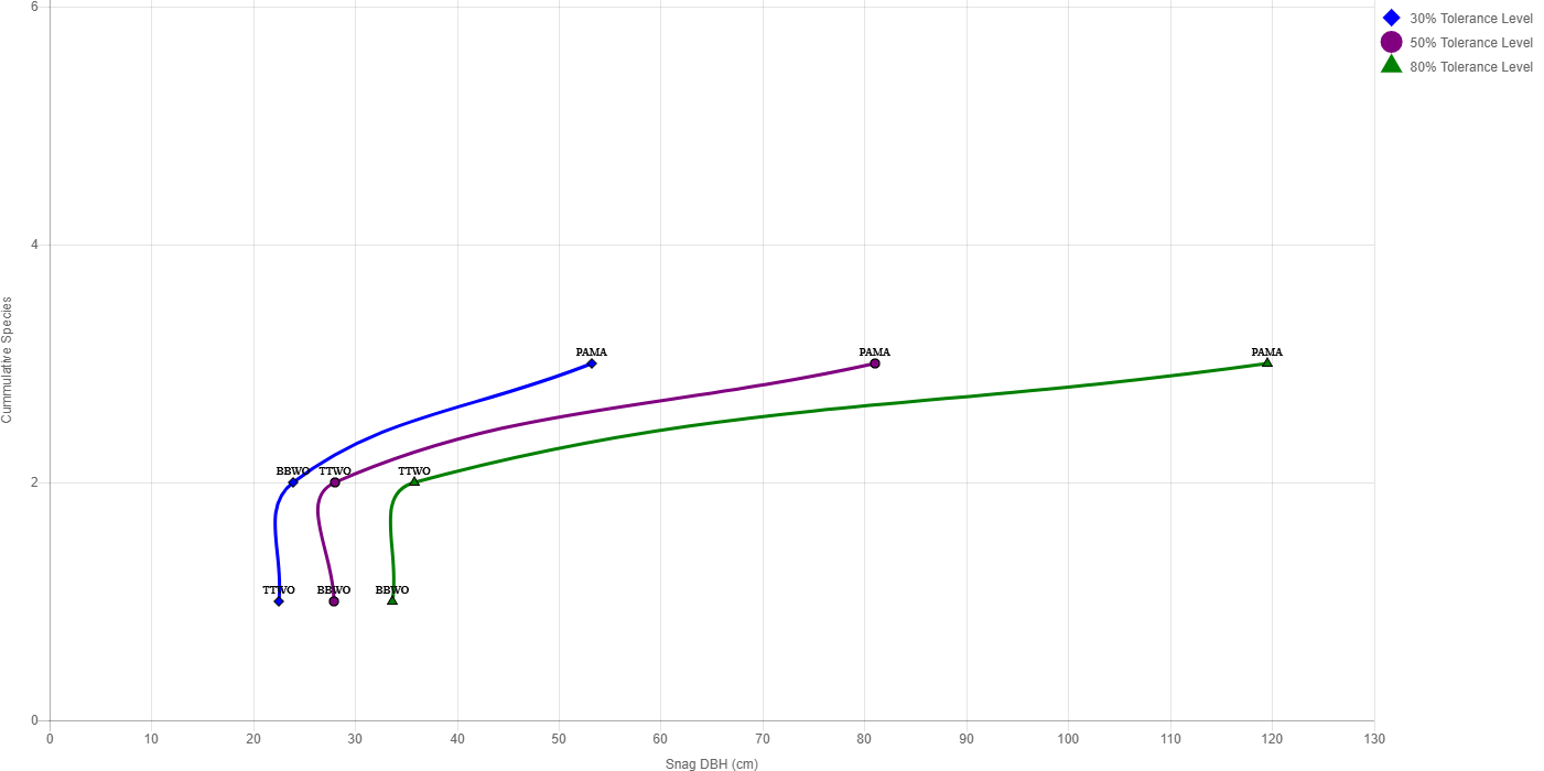
In the wildlife species snag density graphs, the lower curve pertains to 30% of the population, the middle curve 50%, and the top curve 80%. For example, in the snag density graph above (for illustration only), the points labeled DOSQ refers to Douglas' squirrel. On the 30% tolerance level curve, the DOSQ point is interpreted as follows: 30% of DOSQ (at least in the population studied) use areas which contain densities of snags up to 10 snags/ha; 50% of DOSQ use areas which contain densities of snags up to 25 snags/ha; 80% of DOSQ use areas which contain densities of snags up to 48 snags/ha. Conversely, the higher the snag density, the greater the percentage of a given species' population would provide for; only 30% of the DOSQ population would be provided for in areas with less than 10 snags/ha, but 80% of the population would be provided for in areas with 48 snags/ha. In this way, the three curves can be interpreted as different proportions of populations. Occasionally, the 80% tolerance level may exceed the maximum observation because the 80% level is statistically extrapolated from data on the small, sampled portion of the population to the entire population. See "What is a Tolerance Level?" for more details.
To see the actual data underlying the cumulative species curves in these graphs, click on the "Underlying Wildlife or Inventory Data" buttons above the graph. To properly interpret the graphs, read the interpretation of the data in the Narratives; any limitations of the data are discussed there. In general, however, the graphs can be interpreted as follows. For a given curve (tolerance level), the range of the wildlife-use data among species is from the bottom point on the curve to the top point on the curve. Note that the low point of the curve provides dead wood habitat for just one species. Manage areas with the complete range of dead wood values to provide for all species on the curve.
Tip: A generalized assumption underlying the cumulative wildlife species curves, and our synthesis and management implications of the wildlife data, is that "bigger or more is just as good" - that is, if some wildlife species, for example, is shown by research to use snags up to, say, 30 cm dbh, then we assumed it would also use larger diameter snags as well. The same holds for down wood diameter, snag density, and down wood percent cover. There are major exceptions so it is best to manage for the range of values displayed in the curves.
-
Inventory tables are also associated with each habitat type.
-
Inventory distribution histograms appear by clicking on the "Distribution Histogram" button above the graph.
The inventory distribution histograms display the percent of the plot-sized areas of a given vegetation condition that have various amounts of dead wood (density of snags or percent cover of down wood). The x axis is the density of snags or percent cover of down wood and the y axis is the corresponding percent of the area. Actual percentage values are shown at the top of each vertical bar.
In the example histogram below, the x axis displays snag density classes for snags ≥ 50 cm (19.7 in) dbh. In this example, 23% of the area within the vegetation condition contained no measurable snags ≥ 50 cm dbh. The second bar from the left indicates that 22% of the area within this vegetation condition contains snags up to 5 snags/ha (2 snags/acre). And so on.

-
From the pages showing the cumulative wildlife species curves and inventory data, you can follow links to view the underlying data that went into these curves. Click on the buttons "Underlying Wildlife Data" or "Underlying Inventory Data."
Several more levels of wildlife data are available from the underlying data. One can go all the way to the original piece of data and its reference citation. In this way, the user can see the origin of each data item to determine the appropriateness of considering it for local use.
-
Refer to the Species Code link on the top right of the DecAID homepage for a full description of the crosswalk between the codes, common names, and scientific names.
SOME FINAL MISCELLANEOUS INFORMATION
The DecAID Advisor Web site was constructed to strictly adhere to the regulations for accessibility listed in Section 508 of the American with Disabilities Act. This helps ensure that sight-impaired individuals can access all information on the Web site including text, tables, figures, and all other data. Constructing pages to meet these directives means that the Web pages are very simple in structure, format, and design. We have received suggestions for more complicated ways to access and display the information, but many of these designs would violate Section 508.
LITERATURE CITED
Johnson, D.H. and T. A. O'Neil, ed. 2001. Wildlife-habitat relationships in Oregon and Washington. Oregon State University Press, Corvallis OR. 736 pp.
O'Neil, T. A., D. H. Johnson, C. Barrett, M. Trevithick, K. A., Bettinger, C. Kiilsgaard, M. Vander Heyden, E. L. Greda, D. Stinson, B.G. Marcot, P. J. Doran, S. Tank, and L. Wunder. 2001. Matrixes for wildlife-habitat relationships in Oregon and Washington. CD-ROM. in: D. H. Johnson and T. A. O'Neil, ed. Wildlife-habitat relationships in Oregon and Washington. Oregon State University Press, Corvallis OR.
Spies, T.A., J.F. Franklin, and T.B. Thomas. 1988. Coarse woody debris in Douglas-fir forests of western Oregon and Washington. Ecology 69:1689-1702.
Developed or Updated:
Bruce G. Marcot (Developed 10 December 2002)
Kim Mellen-McLean (Updated January 2009 with Barbara Webb Updated December 2013)
Barbara Webb, Steve Acker, Barbara Garcia (Updated August 2017)