Wildlife Tolerance Level Analysis for Salvage Sales
Objective of a Wildlife Tolerance Level Analysis
While a distribution analysis compares current dead wood condition to reference conditions, as represented by the vegetation inventory data, a wildlife tolerance level analysis assesses how wildlife species are affected by the amount of dead wood across the landscape. The closer the current conditions are to reference conditions the higher the likelihood that adequate habitat is being provided for dead wood associated species and processes. However, some species will be affected differently than others as current conditions depart from reference conditions.
A wildlife tolerance level analysis can be conducted for snags or for down wood.
First Step - Determine the Analysis Area
This should be the same Analysis Area used in the Distribution Analysis.
The analysis area should be large enough to represent the variation in snag habitat and distribution from which the inventory data were collected. If this is not possible, a comparison between the project area and the inventory data is not appropriate.
Salvage sales after stand-replacing disturbances are a special situation. Larger fires and insect outbreaks can skew the current conditions, even at the scale of a watershed (10th field HUC), to the point that current conditions in your analysis area no longer represent habitat conditions in the area in which the inventory data were collected. At a watershed scale it may appear that there is an excess of dead wood because many disturbances are as large, or larger, than the watershed scale. But, it may still be a rare occurrence at the regional or sub-regional scale, the scale at which the vegetation data were collected. For this reason, the analysis area for a salvage sale needs to be developed following the process in Determining Size of Analysis Area.
Region-wide Distribution Analysis
The regional Distribution Analysis provides information that can be used in a wildlife tolerance level analysis. This is noted in the individual steps that follow.
Steps 1-4 of a distribution analysis, as described below, have been run for all Forest Service lands in Region 6 using the 2012 GNN data and updated for large fires (>1,000 acres). These data can be used as is and clipped to your forest boundary or watershed.
The region-wide analysis is available with or without buffering for roads. For the outputs with buffering for roads, snag densities were reduced by 40% within 50 meters of roads to account for falling of hazard trees, firewood cutting, etc., as per Bate et al. (2007), and Wisdom and Bate (2008). Determining which layer to use will depend on the extent of firewood cutting along roads in your area.
The user will still need to:
- identify the Wildlife Habitat Types in the analysis area as described in Step 2.
- determine the HRV% for each Successional Structure Class as described in Step 3.
- complete steps 5 and 6.
Instructions for DecAID Regional Analysis, summary template, and distribution analysis template.
To access the analysis go to the Region-wide Distribution Analysis section of the Links to Useful Information section on the main page of this web site.
A webinar has been developed to demonstrate the use of the Region-wide Distribution Analysis.
Wildlife Tolerance Level Analysis
A wildlife tolerance level analysis estimates what percent of the landscape provides habitat for varying species at each tolerance level. This analysis can be conducted for snags and down wood. Below are instructions on how to perform a wildlife tolerance level analysis for a project. A snag analysis is outlined; a down wood analysis would follow the same steps.
Step 1:Data Collection: Determine current snag and down wood distribution across the landscape
This is the same as Step 1 in a Distribution Analysis.
This step has been completed for the entire region in the Region-wide Distribution Analysis. See "Distribution Analysis" link in table 3 of the Guide. The region-wide analysis used GNN data circa 2012. The data have been updated for large fires (>1,000 acres) through 2014 using RAVG maps (http://www.fs.fed.us/postfirevegcondition/index.shtml). See the DecAID Metadata for a list of fires included in the regional analysis. If other disturbances or treatments have occurred in the analysis area since 2012, the dead wood data should be updated prior to conducting a Distribution Analysis. The following are examples of the types of disturbances and treatments that have not been incorporated into the Region-wide Distribution Analysis:
- Disturbances:
- Fires occurring in 2015 and beyond
- Insect and disease activity since 2012
- Past fires not included on RAVG maps (usually <1,000 acres)
- Treatments since 2012
- Salvage sales
- Hazard/danger tree treatments
- Fuels reduction treatments
Here are some sources of information that are available to update the data:
- GIS mapping of various forest stands based on past management can be used to modify snag and down wood densities as needed. Some examples of possible categories are:
- Recent fires create varying densities of snags depending on fire intensity and severity. There are several sources for data on fires. An ArcGIS application is available that uses RAVG maps to update the snag densities in the Regional Distribution Analysis. See the Wildfire maps section of the Links to Useful Information section on the main page of this web site.
- Areas of high snag densities due to other disturbances (e.g. insect infestations where high mortality occurred, areas of root rot, etc.). Region 6 conducts annual aerial surveys of insect- and disease-caused mortality and most National Forests should have this information available in their GIS systems. If not, it can be downloaded from the RO Forest Health Protection website (Aerial Survey Data). These data can be used to help determine areas with high levels of mortality. Annual surveys only calculate "new" dead based on changes in foliage color, so there is a need to overlay multiple years of aerial data. Using 5 to 10 years of aerial data may better reflect existing conditions. If you need assistance in interpretation of the data or in converting data to cumulative numbers of dead trees per acre, contact Ben Smith (bsmith02@fs.fed.us)(WA), Bob Schroeter (rschroeter@fs.fed.us)(OR), or Zach Heath (zheath@fs.fed.us) for assistance in interpreting the data appropriately. Forest Service researchers have been field testing the accuracy of the aerial survey data and their preliminary conclusions suggest that surveys underestimate snag levels. At this time, a general "rule of thumb" is to multiply the reported values by 3.
- Data for recent treatments from project implementation can be found in your local FACTS database.
- Roads have been buffered in the Region-wide Distribution Analysis using a regional roads layer. A local roads layer could be used to more accurately buffer roads. For those who prefer to run the analysis with local data instead of regional data, an Arc Toolbox is available at: T:\FS\Reference\GeoTool\r06\Toolbox\DecAID\R6_DecAIDTbox_huc10.tbx OR Download here: DecAID Tools
- Developed recreation sites, administrative sites, etc. where hazard tree removal has reduced snag levels based on the local Forest policy. This area can be determined by calculating the distance from each site. The resulting acreage can be assigned a snag density.
- Ground surveys - A good methodology can be found in Bate et al. 1999 http://www.fs.fed.us/pnw/pubs/gtr_425.pdf
Step 2:Determine Which Species Should be Addressed for This Project
Begin by looking at the wildlife information and data available for the vegetation type being analyzed. The best place to start is under the INTRODUCTION TO AVAILABLE DATA - Wildlife data section of the Summary Narrative [Level 3] for the Vegetation Condition that applies to your analysis area. If there are data available and summarized for dead wood associated MIS species, species of concern, TES species, focal species, or any other species that should be addressed to support the analysis, the Wildlife Tolerance Level Analysis may be considered for the project. For those species which are not represented in the cumulative species curves, additional data may be available that can assist with the analysis. Additional studies will be mentioned in the same section of the Summary Narrative. A more qualitative assessment can be done for those species.
Step 3:Determine What the Tolerance Levels are for the Species
Refer to the Synthesized Data on Snag Density tables for Post-fire Habitats in DecAID, (e.g. Table EMC_PF.sp-3) to determine snag density tolerance levels. Determine what the snag density is for each wildlife tolerance level for the species being addressed. Develop a table to display this information. Develop a similar table for down wood habitat where data are available.
TIP: Make sure that you are comparing acres to acres or hectares to hectares, as well as inches to inches and cm to cm. See Metric Conversions for English to metric conversion factors.
Conversion Widget
Example of Wildlife Tolerance Level Analysis
Table 1. Snag densities for wildlife species using post-fire habitats at 30, 50, and 80 percent tolerance level for snags >10"dbh. DecAID Table EMC_PF.sp-3.
| Wildlife Species | 30% Tolerance level (#snags/acre) based on wildlife data in DecAID |
50% Tolerance level (#snags/acre) based on wildlife data in DecAID |
80% Tolerance level (#snags/acre) based on wildlife data in DecAID |
|---|---|---|---|
| Black-backed Woodpecker (BBWO) | 55.1 | 75.8 | 115.9 |
| Hairy Woodpecker (HAWO) | 38.5 | 62.3 | 98.6 |
| Lewis's Woodpecker (LEWO) | 24.6 | 42.3 | 69.7 |
| Mountain Bluebird (MOBL) | 37.6 | 62.2 | 99.6 |
| Northern Flicker (NOFL) | 24.6 | 47.2 | 81.8 |
| Western Bluebird (WEBL) | 28.0 | 49.1 | 81.0 |
| White-headed Woodpecker (WHWO) | 0.0 | 39.4 | 116.6 |
Table 2. Snag densities for wildlife species using post-fire habitats at 30, 50, and 80 percent tolerance level for snags >20"dbh. DecAID Table EMC_PF.sp-3.
| Wildlife Species | 30% Tolerance level (#snags/acre) based on wildlife data in DecAID |
50% Tolerance level (#snags/acre) based on wildlife data in DecAID |
80% Tolerance level (#snags/acre) based on wildlife data in DecAID |
|---|---|---|---|
| Lewis's Woodpecker (LEWO) | 0.0 | 6.1 | 20.0 |
| Mountain Bluebird (MOBL) | 0.0 | 12.2 | 37.4 |
Step 4:Build A "Current Condition" Histogram to Display the Amount of Landscape in Each Wildlife Tolerance Level
For Low or Moderate Risk projects (i.e., smaller salvage sales) the graphs in the Distribution Analysis spreadsheet templates can be used to assess the affects to wildlife species. Follow the instructions that accompany the spreadsheets.
Wildlife Tolerance Level Analysis using the Distribution Analysis spreadsheet templates
Select the *_Hist&wildlife tab in the DecAID_DistributionAnalysis *.xlsx for the WHT(s) you are assessing. Figure 1 is an example for the EMC WHT. The red boxes represent wildlife use in post-fire habitat. The green boxes are for forested habitats; they will be helpful for determining effects of salvage over time. Boxes for any species not occurring in the analysis area should be removed from the graph.
Figure 1. Example of Distribution Analysis histogram with wildlife 50% tolerance levels displayed for snags > 10" dbh.
Figure 2. Example of Distribution Analysis histogram with wildlife 50% tolerance levels displayed for snags > 20" dbh.
Interpretation
The following conclusions can be inferred from the information in Figures 1&2, and Tables 1&2 for post-fire habitats:
- Compared to reference conditions, the amount of small snags on the landscape is far below the wildlife 50% tolerance levels, and below the 30% tolerance level for all species except the white-headed woodpecker.
- The amount of large snags on the landscape is far below reference conditions for the 50% and 80% tolerance levels for cavity nesters as a group, Lewis's woodpecker, and norther flicker. The landscape is providing above reference conditions for the 30% tolerance level for all the post-fire species.
- It is likely that there has not been recent stand-replacing disturbances in the analysis area.
The landscape is also below reference conditions for the moderate snag density classes for both small and large snags. The small amount of the landscape with high densities of snags, will contribute to moderate level snag density classes as snags fall over the next decade or so. This is an important consideration when determining the effects of salvage on wildlife habitats.
Detailed Wildlife Tolerance Level Analysis
For High Risk projects (i.e., larger salvage sales) it is recommended that a more detailed analysis be completed as follows.
Using the map created in Step 1 and the information on tolerance level by species from Step 3, calculate how many acres provide those snag densities and down wood percent cover under current conditions and what percent of the landscape those acres represent. This will require skills with GIS. Create a table and/or histogram to display this information.
Acres should just be those within habitat for each individual species. Overlay the species habitat with the snag density data to calculate acres in each tolerance interval. The data to use are the input data used to run the Regional Analysis and are available at: T:\FS\Reference\GeoTool\r06\Toolbox\DecAID\DecAID_data2012 OR Download here: DecAIDData2012.
Table 3. Example of the amount and percent of the analysis area providing snag densities for wildlife species associated with post-fire habitats within four different tolerance intervals (0-30%, 30-50%, 50-80%, and 80-100%) for snags >10"dbh (from table 1). Example Analysis Area =50,000 acres.
| Wildlife Species | Acres (% analysis area) providing habitat at 0-30% tolerance interval | Acres (% analysis area) providing habitat at 30-50% tolerance interval | Acres (% analysis area) providing habitat at 50-80% tolerance interval | Acres (% analysis area) providing habitat at 80-100% tolerance interval |
|---|---|---|---|---|
| Black-backed Woodpecker (BBWO) | 49,500 acres (99%) |
500 acres (1%) |
0 acres (0%) |
0 acres (0%) |
| Hairy Woodpecker (HAWO) | 49,000 acres (98%) |
800 acres (2%) |
200 acres (<1%) |
0 acres (0%) |
| Lewis's Woodpecker (LEWO) | 49,000 acres (98%) |
600 acres (1%) |
300 acres (<1%) |
100 acres (<1%) |
| Mountain Bluebird (MOBL) | 49,000 acres (98%) |
800 acres (2%) |
200 acres (<1%) |
0 acres (0%) |
| Northern Flicker (NOFL) | 49,000 acres (98%) |
700 acres (1%) |
300 acres (<1%) |
0 acres (0%) |
| Western Bluebird (WEBL) | 49,000 acres (98%) |
700 acres (1%) |
300 acres (<1%) |
0 acres (0%) |
| White-headed Woodpecker (WHWO) | 12,000 acres (24%) |
37,700 acres (75%) |
300 acres (<1%) |
0 acres (0%) |
It is important to compare the wildlife data to the inventory data to determine what the area is capable of providing in terms of snag habitat. Use the information from the distribution histograms in DecAID or from the Regional Distribution Analysis Spreadsheets.
Table 4. Example percent of the landscape for reference conditions in the EMC_ECB Wildlife Habitat Type in snag density classes (snags>10" dbh).
| Wildlife Species | 0 snags/acre | 0-6 snags/acre | 6-12 snags/acre | 12-24 snags/acre | 24-36 snags/acre | >36 snags/acre |
|---|---|---|---|---|---|---|
| Percent of Landscape | 18% | 29% | 14% | 20% | 5% | 13% |
Interpretation
The following conclusions about the amount of the analysis area providing post-fire wildlife habitat with adequate densities of snags >10" dbh densities can be inferred from the graph in Figure 1 and Tables 1, 3 & 4:
- Post-fire snag habitat is rare or nonexistent on the landscape at tolerance levels above 50% for all species except the white-headed woodpecker.
- Based on reference conditions, the EMC_ECB Wildlife Habitat should have about 13% of the area with snag densities > 36 snags/acre > 10" dbh. Currently, snag densities that high only occur on about 1% of the Wildlife Habitat Type in the Analysis Area.
Step 5:Assess the effect of project on future snag habitat
Because salvage activities remove large amounts of dead wood, a quantitative assessment is highly recommended for salvage projects and can be accomplished by running the Forest Vegetation Simulator Fire and Fuels Extension (FVS-FFE) with the assistance of your silviculturist or fuels planner. The analysis will show both future stand structure with associated mortality and dead wood dynamics including snag fall and decay. There are several ways to display the results of the analysis. These graphs should have been developed during Step 5 of the Distribution Analysis for Salvage Sales.
Interpretation
Areas providing high density snag habitat after a disturbance are ephemeral. Within 5 to 10 years those areas will be providing moderate levels of snags and down wood as snags killed by the disturbance fall. If the distribution analysis indicates that the area is deficit in moderate snag densities (as is the case in Figures 1 and 2), it may be important to maintain enough of the high density snag pulse to provide areas with moderate snag densities in the near future. Leaving stand-replacing disturbances unsalvaged may be the only feasible way to move the landscape towards reference conditions for moderate snag densities.
Most snags will likely fall before the regenerating stand begins to produce snags through mortality processes. This is referred to as the "snag gap". Salvage will have the effect of increasing the magnitude of the snag gap.
Step 6:Incorporate DecAID Data on size, decay class, etc.
DecAID provides other data on snags and down wood besides snag density:
| Snags | Down wood |
|---|---|
|
|
These data can be used to assist in setting snag and down wood retention guidelines. For example, Figure EMC_PF.sp-1 indicates that at the 80% tolerance level most species use large snags (> 20 inches dbh) for nests and in later seral stages this preference is even more pronounced for roost trees with many species using snags larger than 31 inches dbh (Figure EMC_M.sp-1). Table EMC_ECB_M.inv-1 indicates that these large snags are rare, making up just 4% of all snags surveyed on the unharvested vegetation inventory plots in this habitat type. This information illustrates the value in retaining the largest snags during harvest activities.
Figure EMC_PF.sp-1. Mean height of trees and snags used by wildlife species or groups in Eastside Mixed Conifer Forest Wildlife Habitat Type. Tree heights are weighted means for trees and snags across studies with the same species and tree use.
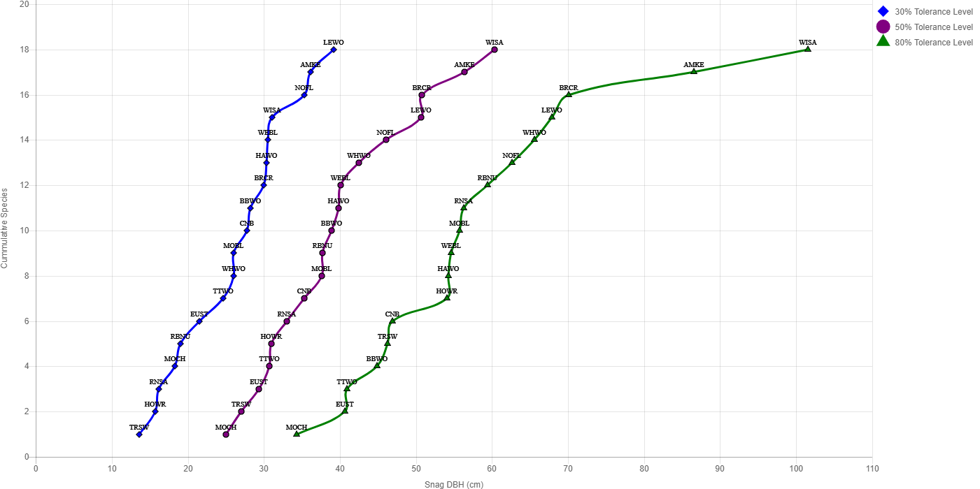
Figure EMC_M.sp-1. Cumulative species curves for snag/tree dbh (cm) used for nesting or denning for 30%, 50%, and 80% tolerance levels in the Eastside Mixed Conifer Forest Wildlife Habitat Type for the Mid Structural Condition Class.
Table EMC_ECB_M.inv-1. Distribution of snag sizes on unharvested forest inventory plots (n=754) in the EMC_ECB_M Vegetation Condition.
| Snag dbh (cm) | % snags (> 25.4 cm) in size class1 | % of area with snags in size class2 |
|---|---|---|
| < 25.42 | N/A | 21 |
| 25.4 - 49.9 | 77 | 63 |
| 50 - 79.9 | 20 | 45 |
| ≥80 | 4 | 36 |
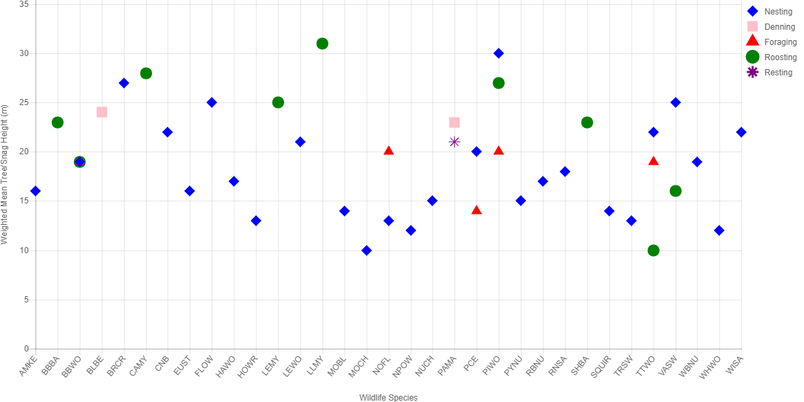
Other data indicate the importance of retaining and recruiting tall snags for roosting bats and pileated woodpeckers (Figure EMC.sp-8).
Figure EMC.sp-8. Mean height of trees and snags used by wildlife species or groups in Eastside Mixed Conifer Forest Wildlife Habitat Type. Tree heights are weighted means for trees and snags across studies with the same species and tree use.
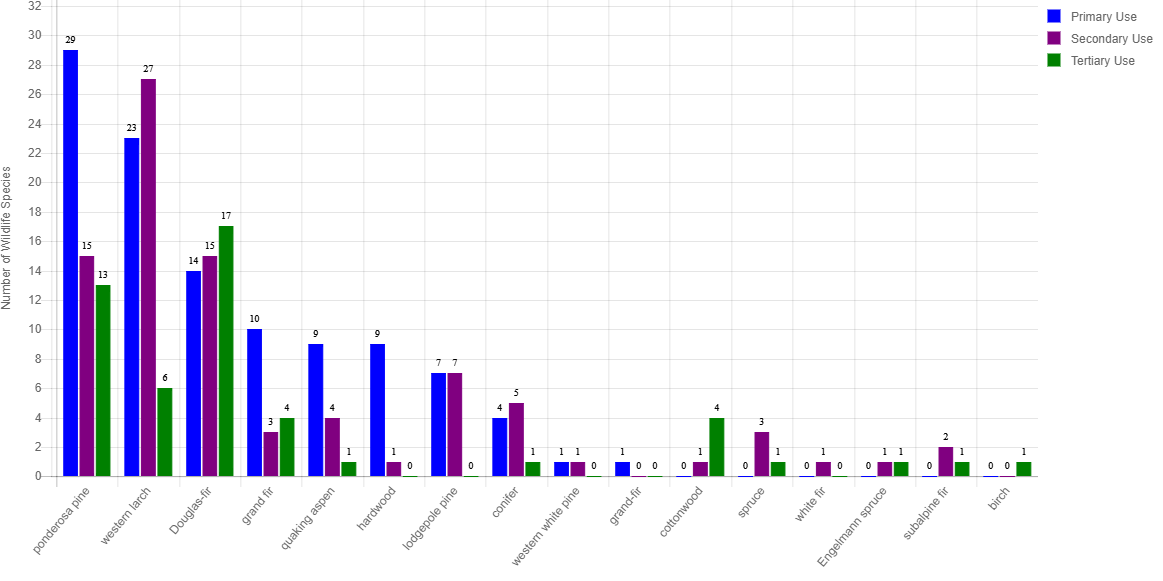
Data showing which trees species are used by snag associated wildlife are also available (Figure EMC.sp-9). This information can be used to determine priority snag or down wood species to emphasize in dead wood retention guidelines.
Figure EMC.sp-9. Number of wildlife species or groups using different tree/snag species in Eastside Mixed Conifer Forest Wildlife Habitat Type.
There is additional discussion on the importance of hollow trees nd logs to a variety of wildlife species. They are especially important roosting and denning structures which take centuries to develop, thus they are important to protect where they exist.
There is a discussion in the Summary Narratives under the section: Considerations for developing, creating and retaining decayed wood elements, which also provides some valuable information that can assist in developing dead wood retention guidelines and marking guidelines.
Step 7:Discuss the "So What" Questions.
For Example:
- How well are wildlife species' needs being met in the analysis area?
- If the species is dependent on large snags and the analysis area is deficient in large snags, how do you move towards getting more? What kind of effect does this have on this wildlife species?
- Is there the need or desire to move part of the landscape towards increasing the wildlife tolerance level for a wildlife species?
- How do the alternatives compare in terms of providing habitat now and in the future?
Snag densities and down wood percent cover are often higher at sites used by wildlife than would be indicated by the use of inventory data alone. Wildlife species may be selecting for clumps of snags around nest sites, dens, etc. which are areas represented by the wildlife species data. These higher density clumps (in relation to inventory data) need to be provided somewhere on the landscape. The vegetation inventory distribution histograms (from unharvested plots) can give clues as to what proportion of the landscape would be expected to provide these high density clumps snags. Graphs like Figure 1 above, are a good way to display which snag density classes may be in excess or deficient on the landscape and which species are affected.
Species home range information, combined with the inventory distribution data, can help determine number and sizes of patches of various snag densities distributed across the landscape that will provide high quality habitat. In this way prescriptions and project design can better accommodate species habitat provisions.
References
Bagne, Karen E., Kathryn L. Purcell, John T. Rotenberry. 2008. Prescribed fire, snag population dynamics, and avian nest site selection. Forest Ecology and Management 255:99-105.
Bate, Lisa J.; Garton, Edward O.; Wisdom, Michael J. 1999. Estimating snag and large tree densities and distributions on a landscape for wildlife management. Gen. Tech. Rep. PNW-GTR-425. Portland, OR: U.S. Department of Agriculture, Forest Service, Pacific Northwest Research Station. 76 p.
Mellen-McLean, Kim, Bruce G. Marcot, Janet L. Ohmann, Karen Waddell, Susan A. Livingston, Elizabeth A. Willhite, Bruce B. Hostetler, Catherine Ogden, and Tina Dreisbach. 2012. DecAID, the decayed wood advisor for managing snags, partially dead trees, and down wood for biodiversity in forests of Washington and Oregon. Version 2.2. USDA Forest Service, Pacific Northwest Region and Pacific Northwest Research Station; USDI Fish and Wildlife Service, Oregon State Office; Portland, Oregon. http://www.fs.fed.us/r6/nr/wildlife/decaid/